15 Displaying Graphics

15.1.1 Section Tree and Solution Data Tree

The core workflow in the Visualization Tab relies on two synchronized hierarchical tree structures that govern spatial domain selection and dataset mapping:

• Section Tree: Displays the spatial partitioning of the computational domain, listing all geometric entities, boundary patches (e.g., inlets, outlets, viscous walls), symmetry planes, and volumetric cell zones. Users can toggle individual sections on or off to isolate specific surfaces for graphic rendering.

• Solution Data Tree: Contains the active flow variables computed by the solver, categorized into fundamental thermodynamic properties (e.g., static pressure, density, static temperature), velocity field scalars (e.g., velocity magnitude, Mach number), turbulence transport scalars (), and species/dispersed-phase concentrations.

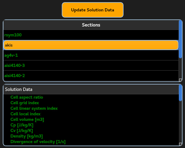
Combining selections from the Section Tree and the Solution Data Tree dynamically maps the target scalar dataset onto the chosen spatial domain, triggering instantaneous 2D/3D contour updates in the graphics viewport.

Leveraging the asynchronous communication architecture between the NeuralFlow solver kernel and the GUIX-H graphical user interface, real-time data transfer and dynamic case setup modifications can be executed seamlessly without interrupting an active simulation run. Clicking the Update Solution Data button queries the solver for the latest iteration dataset, instantly refreshing the available flow variables within the interface and updating all active 2D/3D field contours and visualization pipelines in real time.

15.1.2 Scalar Visualization

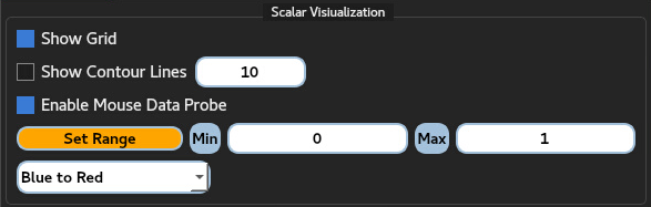
The Scalar Visualization sub-tool generates continuous or banded color contour maps over selected geometric surfaces and interior zones. Users can customize color palettes (e.g., Blue to Red, Rainbow, X-Ray View etc.), adjust scalar legend ranges (auto-scaling or fixed manual limits), show contour lines and grid, and enable mouse data probe.

15.1.3 Scalar Line Plot

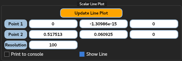
The Scalar Line Plot functionality enables quantitative 1D linear data probing across selected 2D/3D flow fields. Users define a line probe in 3D space by specifying start and end point coordinates and alongside spatial sampling resolution, evaluating the selected scalar field along the defined line segment and rendering a real-time line graph of the variable value versus normalized curvilinear distance.

The control panel incorporates the following user inputs and visualization options:

• Point 1 & Point 2 Coordinates: Specify the Cartesian coordinates for the starting location and ending location of the 1D probe vector within the computational domain.

• Resolution: Defines the total number of discrete sampling points (e.g., ) along the line segment for interpolating field data from surrounding finite-volume cells.

• Update Line Plot: Triggers the numerical sampling routine along the line probe and updates the active 2D scalar distribution plot.

• Print to console: When checked, streams the sampled spatial coordinates and corresponding scalar values directly to the Message View console for numerical logging and rapid data verification.

• Show Line: Toggles the interactive 2D/3D rendering of the line segment within the main graphics viewport, enabling visual confirmation of the probe’s alignment relative to domain boundaries and shock structures.

15.1.4 Threshold

The Threshold filtering tool extracts and displays sub-regions of the computational domain where a selected scalar variable falls within user-specified minimum and maximum numerical bounds.

15.1.5 Slice

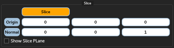
The Slice tool generates 2D planar cutting planes through 3D volumetric unstructured meshes to expose internal flow structures without requiring geometry partitioning:

• Plane Geometry: Planar slices can be positioned arbitrarily by defining an origin point and a normal vector , or aligned with principal Cartesian axes (, , or planes).

• Contour Integration: Real-time scalar contour rendering is automatically mapped onto the dynamic cutting plane as the user translates or rotates the slice interactively through the 3D domain.

• Applications: Crucial for inspecting internal flow features, such as vortex core breakdown inside air intakes, combustion chamber thermal fields, and secondary flow patterns inside complex ducting.

15.1.6 Export VTU File

The Export VTU File feature provides external data interoperability by exporting selected mesh geometry and corresponding field data into the VTK Unstructured Grid XML format (.vtu):

• Export Scope: Users can export full 2D/3D volumetric fields and isolated surface boundary patches (Zone VTU) along with all available scalar and vector fields. All zones checked in Monitor Tool –> Zone VTU Tool are automatically exported when the button is clicked.

• External Integration: Ensures seamless compatibility with industry-standard external post-processing and advanced visualization tools, such as ParaView, VisIt, and custom Python VTK routines.

15.2.1 Available Integral Types

The solver supports twelve specialized surface integration routines:

• Mass Flow Rate [kg/s]: Computes the net continuous gas-phase mass flux across the selected surface :

• Pressure Force [N]: Evaluates the net force vector resulting from static pressure acting normal to the surface, adjusted for ambient reference pressure ():

• Shear Force [N]: Integrates the viscous wall shear stress tensor () over the surface area to determine skin-friction resistance:

• Total Force [N]: Sums the net pressure and viscous shear forces acting on the selected boundary ().

• Moment [Nm]: Calculates the vector moment resulting from surface forces about a specified spatial reference center ():

• Momentum [N]: Computes the convective momentum flux tensor integrated across flow boundaries:

• Average Total Pressure [Pa]: Evaluates the mass-weighted average total pressure () across the selected surface, crucial for total pressure loss calculations in internal flow ducts and intakes.

• Average Total Temperature [K]: Computes the mass-weighted average total temperature (), providing energy transport insights across boundaries.

• Particle Mass Flow Rate [kg/s]: Integrates the mass flux strictly for the dispersed particulate or droplet phase across the selected surface when multiphase transport models are active.

• Center of Pressure [m]: Determines the spatial coordinate vector () where the net aerodynamic line of action intersects the geometry, eliminating net pressure moments.

• Cd (Drag Coefficient): Computes the non-dimensional drag coefficient by projecting total aerodynamic force onto the specified reference directional axis:

• Cl (Lift Coefficient): Evaluates the non-dimensional lift coefficient by projecting total aerodynamic force onto the direction normal to the reference drag axis:

15.2.2 Reference Values and Parameter Dependence

The input fields within the Reference Values section are selectively utilized depending on the mathematical formulation of the chosen integral type. While basic conservation fluxes do not require reference conditioning, forces, moments, and dimensionless coefficients depend strictly on these parameters:

• Scalar Reference Inputs:

  • Ref Pressure [Pa]: Subtracted from absolute static pressure to calculate net gauge pressure forces (). Ignored during shear force or pure flux integrations.

  • Ref Area [m]: Normalization area () used exclusively for non-dimensionalizing forces into Cd and Cl.

  • Ref Density [kg/m]: Dynamic pressure denominator density () utilized exclusively in Cd and Cl formulas.

  • Ref Velocity [m/s]: Freestream reference velocity () utilized exclusively in Cd and Cl formulas.

• Vector Reference Inputs:

  • Ref Position [m] : Defines the moment origin point () for Moment and Center of Pressure calculations. Ignored for force and flux integrals.

  • Ref Axis : Specifies the directional unit vector () representing the primary flow or drag direction. Crucial for projecting total forces into Cd, Cl, and Center of Pressure components.

Note. Input Independence Notice: For pure transport integrals—such as Mass Flow Rate, Particle Mass Flow Rate, Momentum, and Shear Force—all scalar and vector reference inputs are completely bypassed by the integration kernel.