14 Solution Control
The Solution Control module governs the numerical integration schemes, temporal discretization, CFL stability criteria, convergence criteria, and linear solver acceleration algorithms in NeuralFlow. It provides full operational control over both steady-state pseudo-time marching and time-accurate transient simulations.
14.1 Standard Solver Control Options
The Standard Solver Control Options interface
configures time-integration algorithms, CFL stability limits,
preconditioning parameters, convergence thresholds, and acceleration
routines. The standard solver control options can be accessed via the
Solution Control Tool
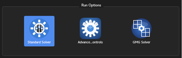
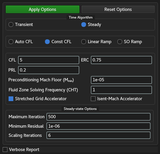
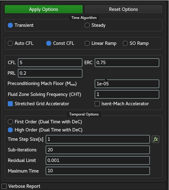
Figure 14.2 and Figure 14.3 illustrate the interface configurations for steady-state and transient solver modes, respectively.
14.1.1 Time Algorithm Selection and CFL Controls
At the top of the interface, users select the primary time-marching paradigm under Time Algorithm:
Steady: Employs local pseudo-time stepping to march the solution toward a stationary asymptotic convergence state.
Transient: Activates time-accurate physical transient integration, enabling sub-iterative dual-time stepping schemes.
Stability and convergence rate are strongly governed by the Courant-Friedrichs-Lewy (CFL) condition. Users can choose among four distinct CFL Ramping Modes:
Auto CFL: Dynamically adjusts the local CFL number based on residual reduction history and solution gradient stability.
Const CFL: Maintains a user-defined constant CFL value throughout the entire simulation run.
Linear Ramp: Linearly increases the active CFL number from a low initial baseline to the target CFL value over a specified initial iteration window, preventing early solution divergence.
SO Ramp: Applies a smooth, second-order S-curve (sigmoidal) ramping profile to softly transition the CFL number, ideal for highly stiff or strongly shock-dominated compressible flows.
14.1.2 Global Numerical and Acceleration Parameters
The core numerical stability controls apply to both steady and transient execution modes:
CFL: Defines the target Courant-Friedrichs-Lewy number. Higher CFL values increase numerical pseudo-time step sizes and accelerate convergence, but require robust grid quality and physics initialization.
ERC (Explicit Relaxation Coefficient): Controls explicit parameter damping and updates for conservation equations, providing numerical stability in high-gradient shock or boundary-layer regions.
PRL (Pseudo Residual Limit): Specifies upper bound limits on local cell update increments to prevent unphysical solution spikes (e.g., negative pressure or temperature bounds) during early iteration stages.
Preconditioning Mach Floor (
): Sets the low-Mach cut-off limit ( ) for time-derivative preconditioning. This eliminates system stiffness and maintains matrix condition numbers when solving low-speed or near-stagnation compressible flows (e.g., ). Fluid Zone Solving Frequency (CHT): Specifies the execution frequency ratio of the fluid domain solver relative to solid conduction updates during Conjugate Heat Transfer (CHT) simulations. A value of
evaluates fluid dynamics at every time step/iteration. Stretched Grid Accelerator: Toggles local pseudo-time step scaling on highly anisotropic, high-aspect-ratio boundary layer elements, mitigating stiffness induced by extremely small wall-normal cell heights.
Isent-Mach Accelerator: Activates local convergence acceleration based on local isentropic Mach number relationships, speeding up steady-state trans-sonic and supersonic flow updates.
14.1.3 Steady-State Options
When Steady algorithm mode is active, the Steady-state Options sub-panel configures global stopping and scaling criteria:
Maximum Iteration: Sets the maximum allowable pseudo-time iterations before terminating the solver run.
Minimum Residual: Defines the absolute convergence stopping threshold. If all scaled governing equation residuals drop below this limit (e.g.,
), the simulation concludes successfully. Scaling Iterations: Specifies the initial iteration window used to compute baseline residual normalization factors. Raw unscaled residuals computed during these iterations serve as the reference denominator for relative residual tracking.
14.1.4 Temporal Options for Transient Simulations
When Transient algorithm mode is enabled, the Temporal Options panel configures physical time discretization and dual-time stepping mechanics:
Time Discretization Schemes:
First Order (Dual Time with DeC): First-order temporal integration utilizing Deferred Correction (DeC) dual-time stepping for robust transient stability.
High Order (Dual Time with DeC): High-order time-accurate integration utilizing Deferred Correction (DeC), recommended for resolving transient vortex shedding, acoustics, or unsteady mixing layers.
Time Step Size [s]: Sets the physical time step size (
) in seconds. Clicking the adjacent function button ( fx) allows defining time-varying or expression-based time step functions.Sub-iterations: Defines the maximum number of inner pseudo-time sub-iterations executed to converge the non-linear governing equations within each physical time step.
Residual Limit: Specifies the inner sub-iteration convergence target. If inner residuals drop below this threshold within a physical time step, the solver advances immediately to the next physical time level without completing all remaining sub-iterations.
Maximum Time: Sets the total physical simulation stopping time in seconds.
14.1.5 GUI Execution and Console Output
Apply Options / Reset Options: The green Apply Options button commits user inputs to the active solver memory state. Reset Options restores all fields to their previously saved or default values.
Verbose Report: Enabling this checkbox streams detailed low-level matrix diagnostics, preconditioner status, and convergence metrics to the terminal and solver log files for advanced troubleshooting.
14.2 Advanced Solver Control Options
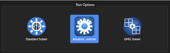
The Advanced Controls menu provides detailed settings for linear solver selection, numerical tolerances, and preconditioning strategies.
14.2.1 Solver Type
Select the primary linear solver method:
Preconditioned Krylov Subspace (PCKSS): Employs Krylov subspace methods coupled with preconditioning (default choice).
Aggregation Algebraic Multigrid (AAMG): Uses algebraic multigrid methods based on aggregation for rapid error reduction across multiple scales.
AAMG Preconditioned Krylov Subspace (AAMGKSS): Combines AAMG preconditioning with Krylov subspace acceleration.
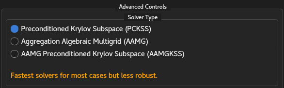
Note: These solvers are the fastest options for most cases, but they may be less robust under severely ill-conditioned conditions.
14.2.2 Preconditioned Krylov Subspace (PCKSS) Solver Options
When Preconditioned Krylov Subspace (PCKSS) is selected, the global convergence control options and PCKSS-tailored preconditioning and sub-solver parameters become configurable. PCKSS algorithms represent the fastest choice for well-behaved or moderately coupled systems, though selecting the appropriate preconditioner and Krylov variant is essential for maintaining solver robustness in stiff CFD applications.
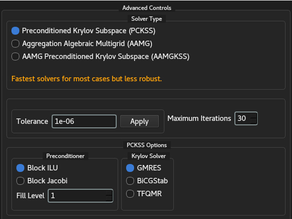
Note. PCKSS options generally offer the highest computational speed for standard flow problems, but may require switching to AMG-based solvers under severe mesh distortion or extreme physical non-linearities.
14.2.2.1 Convergence Parameters
Tolerance: Sets the relative residual convergence target for the linear solver (default:
). Click Apply to confirm modifications. Maximum Iterations: Defines the allowable linear solver iteration limit per global non-linear iteration (default:
).
14.2.2.2 Preconditioner Options
Preconditioners transform the linear system
Block ILU (Incomplete LU Factorization):
Mechanism: Computes an incomplete lower-upper block factorization, discarding fill-in elements beyond a specified structural level.
Pros: Provides high preconditioning quality, dramatically reducing total Krylov iterations. Highly robust for strongly coupled multi-variable systems and steep boundary layer gradients.
Cons: Higher memory footprint and factorization setup cost per outer step compared to block-diagonal methods. Exhibits lower intrinsic parallel scalability due to serial block dependencies.
Recommended Usage: Default and primary choice for complex, coupled, or strongly convection-dominated compressible flow regimes.
Block Jacobi:
Mechanism: Inverts local diagonal matrix blocks independently while neglecting off-diagonal coupling between subdomain blocks.
Pros: Extremely fast per-iteration execution and minimal memory overhead. Achieves near-ideal parallel scaling across high MPI core counts due to negligible inter-process communication latency.
Cons: Weak preconditioning capacity. Requires significantly more Krylov sub-iterations to converge and may stall or diverge on ill-conditioned systems.
Recommended Usage: Best suited for well-conditioned linear systems (e.g., pure thermal conduction or smooth subsonic flows), isotropic fine meshes, or massively parallel jobs where communication overhead is the dominant bottleneck.
Fill Level:
Mechanism: Controls the allowable fill-in depth of preconditioning matrix (default:
). Impact: Increasing the fill level (e.g.,
or ) retains higher-order neighbor couplings, producing a stronger preconditioner that reduces linear solver iteration counts. However, higher fill levels exponentially increase memory footprint and setup time. A value of provides an optimal balance between solver stability and memory economy for most CFD cases.
14.2.2.3 Krylov Solver Options
Krylov subspace solvers construct iterative approximations over expanding projection spaces generated by the preconditioned coefficient matrix.
GMRES (Generalized Minimal Residual):
Mechanism: Utilizes the Arnoldi process to build an orthonormal basis, minimizing the residual norm over the Krylov subspace at every step.
Pros: Guarantees monotonic residual reduction for general non-symmetric matrices. Highly stable and resilient against severe flow non-linearities and strong shock waves.
Cons: Memory footprint and orthogonalization cost grow linearly with iteration count, requiring periodic restarts or storage limits.
Recommended Usage: Default recommendation for general compressible flows, trans-sonic/supersonic aerodynamics, and coupled conjugate heat transfer problems.
BiCGStab (Biconjugate Gradient Stabilized):
Mechanism: Combines standard BiCG Lanczos updates with local steepest-descent residual minimizations, eliminating full basis storage requirements.
Pros: Maintains a low, constant memory footprint regardless of iteration count. Offers rapid per-iteration execution times.
Cons: Residual reduction can exhibit severe non-monotonic oscillations or stall if the matrix spectrum contains complex eigenvalues or strong non-normality.
Recommended Usage: Ideal for memory-constrained large-scale meshes or smooth, steady diffusion-dominated problems where GMRES memory overhead becomes prohibitive.
TFQMR (Transpose-Free Quasi-Minimal Residual):
Mechanism: Computes a quasi-minimal residual solution profile derived from Conjugate Gradient Squared (CGS) updates without requiring transpose matrix-vector products.
Pros: Delivers significantly smoother convergence curves than BiCGStab without incurring the heavy memory accumulation of GMRES. Highly effective at smoothing out residual spikes.
Cons: Performs two matrix-vector operations per iteration, making each Krylov step slightly more computationally expensive than BiCGStab.
Recommended Usage: Preferred alternative when BiCGStab exhibits erratic residual oscillations or stalling, but hardware memory constraints prevent allocating a large GMRES Krylov subspace.
14.2.3 Aggregation Algebraic Multigrid (AAMG) Solver Options
When Aggregation Algebraic Multigrid (AAMG) is selected, the solver replaces or enhances standard Krylov projections by constructing a hierarchy of coarser algebraic grids directly from the system matrix coefficients. AAMG groups strongly coupled fine-grid cells into coarse aggregates without requiring geometric mesh hierarchies, efficiently dampening low-frequency error components that stall conventional single-grid iterative solvers.
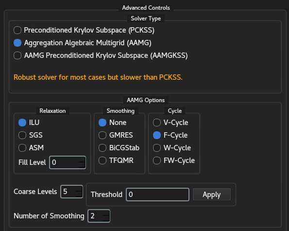
Note. AAMG provides exceptional numerical robustness for ill-conditioned systems, highly stretched boundary layer meshes, and strong physical property jumps. However, its setup overhead and memory footprint make it computationally slower per iteration compared to PCKSS.
14.2.3.1 Relaxation Schemes
Relaxation operators perform pre- and post-smoothing sweeps at each grid level, eliminating high-frequency errors relative to the local grid scale.
ILU (Incomplete LU Factorization):
Mechanism: Applies localized incomplete lower-upper matrix factorizations to smooth residual fields across local cell neighborhoods.
Pros: Highly potent smoother for strongly convective, anisotropic, or directionally coupled flow equations.
Cons: Higher memory consumption and setup time than basic point-relaxation schemes.
Recommended Usage: Default and optimal choice for complex compressible flow simulations with high mesh aspect ratios.
SGS (Symmetric Gauss-Seidel):
Mechanism: Performs alternating forward and backward sweeps over the linear system matrix, ensuring symmetry in the relaxation operator.
Pros: Low computational overhead, zero additional memory allocation, and guaranteed stability for symmetric or weakly non-symmetric operators (e.g., pressure-Poisson or thermal diffusion equations).
Cons: Slower error attenuation on non-symmetric, advection-dominated transport equations.
Recommended Usage: Best suited for diffusion-dominated problems or scalar transport equations on isotropic meshes.
ASM (Additive Schwarz Method):
Mechanism: Decomposes the global matrix into overlapping local subdomains, solving local boundary value problems independently before accumulating updates.
Pros: Superior parallel efficiency across high core-count MPI environments due to localized communication patterns.
Cons: Convergence rate can deteriorate if overlap regions between parallel subdomains are too narrow.
Recommended Usage: Recommended for large-scale distributed-memory parallel runs where global matrix sweeps incur unacceptable communication latencies.
Fill Level:
Mechanism: Defines the structural fill-in level allowed for relaxation (default:
). Impact: Setting
preserves the exact zero-pattern of the coefficient matrix , minimizing memory footprint while maintaining fast smoothing performance.
14.2.3.2 Smoothing Acceleration
In addition to basic stationary relaxations, AAMG allows embedding a Krylov subspace solver as an inner level smoother to handle severe matrix non-normality.
None: Uses standard stationary relaxation sweeps (e.g., pure ILU or SGS) without inner Krylov acceleration (default).
GMRES / BiCGStab / TFQMR: Applies small-step Krylov subspace projections within the multigrid smoothing phase. This stabilizes high-frequency error reduction in regions with steep localized shocks, severe species source terms, or extreme grid skewness.
14.2.3.3 Multigrid Cycle Strategies
The Cycle selection governs the recursive traversal path between fine and coarse algebraic grid levels during each multigrid step:
V-Cycle:
Mechanism: Descends sequentially from the finest mesh down to the coarsest representation and returns directly back to the fine grid.
Pros: Lowest computational cost, minimum memory bandwidth usage, and fastest turnaround per cycle.
Cons: May exhibit slow convergence rates if coarse-grid error corrections are inaccurate.
F-Cycle:
Mechanism: Executes a hybrid traversal strategy, performing an intermediate V-cycle call during the coarsening path before completing the main fine-grid return sweep (default).
Pros: Offers an ideal compromise between the low cost of a V-cycle and the robust error damping of a W-cycle.
Cons: Slightly higher computational overhead per iteration compared to a basic V-cycle.
W-Cycle:
Mechanism: Performs multiple recursive coarse-grid sweeps at every level before returning fine-grid updates.
Pros: Extremely effective at eliminating persistent low-frequency errors on stiff, highly coupled linear systems.
Cons: Significantly higher computational cost and parallel sync overhead per iteration.
FW-Cycle (Flexible W-Cycle):
Mechanism: Dynamically adjusts the coarse level trajectory based on real-time residual reduction metrics.
Pros: Maximizes solver stability on severely ill-conditioned or floating-point sensitive problems.
Cons: Dynamic path evaluation introduces slight algorithmic overhead during coarse grid traversals.
14.2.3.4 Coarsening and Iteration Parameters
Coarse Levels: Specifies the maximum depth of the multigrid hierarchy (default:
). Defines how many successive aggregate grid levels are constructed during setup. Threshold: Sets the relative strength-of-connection criterion used to aggregate matrix entries. Off-diagonal couplings below this threshold are neglected during aggregate formation, controlling grid coarsening geometry. Click Apply to regenerate the algebraic grid hierarchy with updated threshold values.
Number of Smoothing: Sets the number of pre- and post-smoothing relaxation sweeps performed at each grid level (default:
). Increasing this value enhances stability per multigrid cycle at the cost of higher per-iteration compute times.
14.2.4 AAMG Preconditioned Krylov Subspace (AAMGKSS) Options
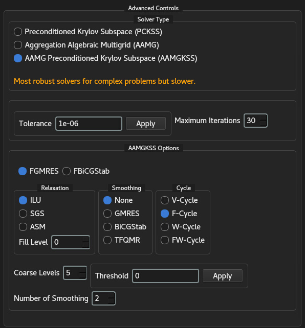
The AAMG Preconditioned Krylov Subspace (AAMGKSS) solver integrates an outer Flexible Krylov subspace iteration with an inner Aggregation Algebraic Multigrid (AAMG) preconditioner. Standard Krylov methods (e.g., GMRES) require a linear, fixed preconditioning operator. Because algebraic multigrid cycles can vary dynamically across outer iterations, flexible Krylov formulations (FGMRES and FBiCGStab) are employed to ensure numerical stability and rigorous outer convergence.
Note. AAMGKSS represents the most robust linear solver configuration available in NeuralFlow. It is specifically designed to overcome extreme stiffness, severe physical property jumps, and highly skewed or distorted meshes where PCKSS and standard AAMG fail. However, it incurs the highest computational cost and memory overhead per iteration.
14.2.4.1 Convergence Parameters
Tolerance: Defines the relative outer residual convergence target (default:
). Click Apply to update this value. Maximum Iterations: Specifies the maximum allowable outer Krylov iterations per non-linear step (default:
).
14.2.4.2 Flexible Outer Krylov Solvers
Standard Krylov solvers assume a stationary preconditioner matrix
FGMRES (Flexible Generalized Minimal Residual):
Mechanism: Extends classic GMRES by storing preconditioned direction vectors at every step, allowing the inner AAMG preconditioner to alter its cycle or smoothing parameters dynamically.
Pros: Guarantees monotonic residual reduction and maximum robustness on severely ill-conditioned linear systems.
Cons: Requires storing both Krylov basis and preconditioned vectors, doubling the memory footprint compared to standard GMRES.
Recommended Usage: Default and primary choice for extreme aerodynamic cases, transonic/supersonic shock interactions, and complex conjugate heat transfer simulations.
FBiCGStab (Flexible Biconjugate Gradient Stabilized):
Mechanism: Formulates a flexible variant of BiCGStab that allows dynamic preconditioning while avoiding full basis orthogonalization.
Pros: Maintains a constant, low memory allocation regardless of outer iteration count, delivering faster per-iteration speed than FGMRES.
Cons: Residual reduction can exhibit non-monotonic oscillations or stall if matrix non-normality is severe.
Recommended Usage: Recommended for large-scale, memory-constrained meshes where AMG robustness is required, but FGMRES memory allocation exceeds system RAM capacity.
14.2.4.3 Inner Multigrid Preconditioner (AAMG) Settings
The sub-panels control the inner AAMG preconditioning operator that acts upon the outer flexible Krylov solver:
Relaxation Operator:
ILU (Incomplete LU Factorization): Applies block ILU smoothing across grid levels.
SGS (Symmetric Gauss-Seidel): Symmetric forward/backward relaxation sweeps; low memory, ideal for symmetric or weakly advective transport operators.
ASM (Additive Schwarz Method): Overlapping domain decomposition relaxation; maximizes scalability in distributed-memory parallel architectures.
The Fill Level parameter (default:
) sets the allowed factorization fill-in depth. Smoothing Acceleration:
None: Uses standard stationary relaxation sweeps during AMG preconditioning (default).
GMRES / BiCGStab / TFQMR: Embeds localized Krylov sub-iterations within the multigrid smoothing phase to suppress high-frequency local errors.
Cycle Strategy:
V-Cycle: Standard fast traversal; lowest computational cost per cycle.
F-Cycle: Hybrid coarsening trajectory; provides optimal balance between execution speed and error attenuation (default).
W-Cycle: Multi-sweep trajectory for stubborn low-frequency error components.
FW-Cycle (Flexible W-Cycle): Dynamically adjusts coarse-grid paths based on localized error metrics.
14.2.4.4 Coarsening and Iteration Parameters
Coarse Levels: Defines the maximum depth of the aggregate grid hierarchy (default:
). Threshold: Controls the strength-of-connection threshold used to cluster fine cells into coarse aggregates. Click Apply to rebuild the aggregate tree after modifying this value.
Number of Smoothing: Sets the number of pre- and post-smoothing relaxation sweeps executed per multigrid level (default:
).
14.3 Geometric Multigrid (GMG) Solver Control Options
Accelerates linear systems convergence by applying restrictive coarser mesh representations. Users can define V, W, or F cycles alongside smoothing algorithms like Gauss-Seidel or Jacobi relaxation.
Note. Development Status Warning: The Geometric Multigrid (GMG) solver is currently non-functional in the present software release. Core framework implementations—including automatic mesh agglomeration, implicit cycle strategies (V-Cycle, F-Cycle, W-Cycle), explicit schemes (Fast Approximate Solver – FAS), and full parallelization—are actively under development and scheduled for integration in upcoming updates.