16 Wall Boundary Layers

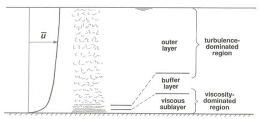
Flow fields near wall boundaries are dominated by viscous forces where flow velocity changes from zero on the wall to the mean free stream velocity away from the wall surface. In fluid mechanics, the boundary layer is the zone where the flow velocity changes from zero to the %99 of the free stream velocity. In turbulent flows, wall boundaries are the main source of turbulence, while, at the same time the dissipation rate is the highest near the wall surfaces due to high viscous forces. For low Re numbers, boundary layers may be fully laminar. For high Re number turbulent flows, laminar zone in the boundary layer becomes thinner. In this respect, turbulent boundary layers are divided into two regions; outer layer and inner layer. In the outer boundary layer, the flow is assumed to be fully turbulent while the inner layer is further divided into three sub-zones; log layer, buffer layer, and viscous zone. In the log layer, flow is equally dominated by viscous and turbulent effects. In the viscous layer, flow is assumed to be fully laminar while the buffer layer is the transition zone between viscous and log layers.

Each layer requires a different numerical approach if a direct numerical simulation (DNS) mesh is not used for these zones. Viscous zones may be easily resolved for many problems, however, for other zones analytical/empirical approaches are required.

For low Re number flows, some turbulence models such as \(k-\omega\) models can be solved to the wall surface with some damping functions accounting for the vorticity vorticity-blocking effect of the solid surfaces. In this case, still, a mesh resolution of \(y^+=1\) is still needed with finely resolved boundary layer mesh. In the case of high Re number flows, a hybrid turbulence model may be used such as SST \(k-\omega\) model, in which, \(k-\varepsilon\) model is used in high Re free flow zones while \(k-\omega\) is used for low Re number near wall zones. This type of approach resolving boundary layer with a proper turbulence model is called Near-Wall Turbulence Modelling (NWTM).

Another approach is to provide semi-empirical boundary conditions for all flow variables effected by the wall boundary. This approach is called Wall Treatment (WT) or Wall Functions method. Wall functions impose values of transported values on the cell centers of the near wall cells. In CMPS, both VWTM and wall functions are used in CMPS for SST \(k-\omega\) method. For \(k-\varepsilon\) only wall function methods must be used.

16.1 Wall Treatment

Wall functions are some type of semi-empirical formulations providing boundary condition-like values for near-wall cell center values. In literature there are mainly two types of wall functions; Standard Wall Functions and Blended Wall Functions (or y+ independent wall functions).

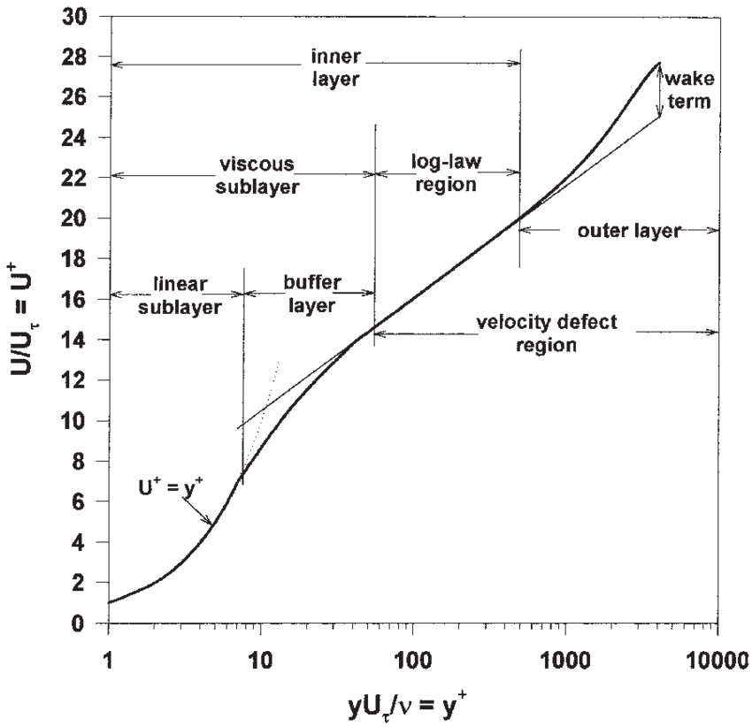
Standard wall functions are only available for the viscous sub-layer and the log layer. Since the viscous sub-layer is assumed to exist for \(y^+<3\), these functions are generally used for \(30<y^+<600\) boundary cell resolutions where the log layer starts. It is generally assumed that a buffer layer exists for \(3<y^+<30\).

\(y^+\) independent wall functions cover all three sublayers up to \(y^+=600\) and enable the use of various size boundary layer meshes with very high or low resolution. These functions automatically adjust if a high-resolution boundary layer solution is required such as at \(y^+=1\).

Wall functions are generally defined in terms of some non-dimensional quantities which are described in the following sections.

16.1.1 Non-dimensional Wall Distance

Non-dimensional wall distance \(y^+\) or simply y plus is defined as; \[ y^+=\frac{y\rho u_*}{\mu}\](16.1) where \(u_*\) is the friction velocity (velocity scale) at the near wall cell described in Section 16.1.5 and \(y\) is the distance to the nearest wall.

16.1.2 Wall Tangential Non-dimensional Velocity

Dimensionless wall tangential component of the velocity \(u\) is given by; \[ u^+=\frac{u}{u_*}\](16.2)

16.1.3 Dimensionless Temperature

\[ T^+=\rho C_p u_*\frac{T-T_w}{q^{''}}\](16.3) where \(q^{''}\) is the wall heat flux and \(T_w\) is the wall surface temperature.

16.1.4 Dimensionless Turbulence Values

Turbul eddy viscosity; \[ \mu_t^+ = \frac{\mu_t}{mu}\](16.4) Turbulent kinetic energy; \[ k^+=\frac{k}{u_*^2}\](16.5) Production of turbulent kinetic energy; \[ P_k^+=\frac{P_k\mu}{\rho u_*^4}\](16.6) Dissipation rate; \[ \varepsilon^+=\frac{\varepsilon\mu}{\rho u_*^4}\](16.7) Specific dissipation rate; \[ \omega^+=\frac{\omega\mu}{\rho u_*^4}\](16.8)

16.1.5 Velocity Scale

Friction velocity represents the value of the velocity component tangent to the wall at near wall cell center. The formulation for this value depends on the used wall function type and \(y^+\) value. Remember that in the case of standard wall functions values for buffer zone are not available.

For standard wall functions; \[ u_*=\begin{cases} \frac{\mu\left|\mathbf{v}_{\text{tang}} \right|}{\rho y} & \text{if }\; y^+<3 \\ \text{invalid} & \text{if }\; 3<y^+<30 \\ C_\mu^{1/4}k^{1/2} & \text{if }\; 30<y^+<600 \end{cases}\](16.9) where \(C_\mu=0.09\) is a model coefficient.

For \(y^+\) independent wall treatment; \[ u_*=\gamma\frac{\mu\left|\mathbf{v}_{\text{tang}} \right|}{\rho y} + \left(1-\gamma \right) C_\mu^{1/4}k^{1/2}\](16.10) where \(\gamma\) is a blending function; \[ \gamma=\exp\left(-\frac{\text{Re}_d}{11} \right)\](16.11) where \(\text{Re}_d\) is the wall distance Reynolds number; \[ \text{Re}_d=\frac{\sqrt{k}d\rho}{\mu}\](16.12)

Wall tangential velocity \(\mathbf{v}_{\text{tang}}\) is calculated as; \[ \mathbf{v}_{\text{tang}}=\left(\mathbf{v}_c - \mathbf{v}_w \right) - \left[\left(\mathbf{v}_c - \mathbf{v}_w \right)\cdot\mathbf{n} \right]\mathbf{n}\](16.13) where \(c\) and \(w\) indicate near cell center and wall surface values, and \(\mathbf{n}\) is wall face normal unity vector.

16.1.6 Velocity Wall Functions

Velocity wall functions provide the distribution of \(u^+\) in a turbulent boundary layer.

For standard wall treatment; \[ u^+=\begin{cases} y^+ & \text{if }\; y^+<3 \\ \text{invalid} & \text{if }\; 3<y^+<30 \\ \frac{1}{\kappa}\ln \left(E^{'}y^+ \right) & \text{if }\; 30<y^+<600 \end{cases}\](16.14) where \(\kappa=0.42\) is the von Karman constant \(E^{'}\) is the modified log law offset defined as; \[ E^{'}=\frac{E}{f}\](16.15) where \(E\) is the log law offset and \(f\) is the roughness function which is 1.0 for smooth surfaces.

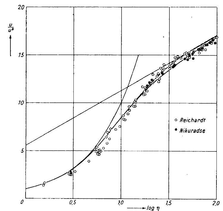
Velocity wall function for \(y^+\) independent treatment based on the paper (Reichardt 1951) is described by; \[ u^+=\frac{1}{\kappa}\ln\left(1+\kappa y^+ \right)+C\left(1-e^{-y^+/y^+_m}-\frac{y^+}{y^+_m} e^{-by^+}\right)\](16.16) where; \[ C=\frac{1}{\kappa}\ln\left(\frac{E^{'}}{\kappa} \right)\](16.17) \[ b=\frac{1}{2}\left(y^+_m\frac{\kappa}{C}+\frac{1}{y^+_m} \right)\](16.18) \[ y^+_m=\max\left[3.0,267\left(2.64-3.9\kappa \right){E^{'}}^{0.0125} \right]-0.987\](16.19)

16.1.7 Temperature Wall Functions

The temperature wall functions describe the distribution of dimensionless temperature \(T^+\) in the turbulent boundary sublayers.

The standard temperature wall function is defined as; \[ T^+=\begin{cases} \text{Pr}y^+ & \text{if }\; y^+<3 \\ \text{invalid} & \text{if }\; 3<y^+<30 \\ \text{Pr}_t\left[\frac{1}{\kappa}\ln \left(E^{'}y^+ \right)+P\right] & \text{if }\; 30<y^+<600 \end{cases}\](16.20) where Pr is the Prandtl number; \[ \text{Pr}=\frac{C_p\mu}{\lambda}\](16.21) where \(\lambda\) is the thermal conductivity. \(\text{Pr}_t=0.85\) is the turbulent Prandtl number. \(\kappa = 0.42\) is the von Karman constant. \(E^{'}\) is defined in Eq. (16.15). \(P\) is a dimensionless parameter known as the \(P\)-function, which accounts for the resistance to heat transfer across the viscous sublayer (Malin 1987). Several sublayer resistance functions are proposed in the literature. In CMPS, the function is taken from (Jayatilleke 1966) and defined as; \[ P=9.24\left[B^{3/4}-1\right]\left[1+0.28\exp\left(-0.007B\right) \right]\](16.22) where \(B=\text{Pr}/\text{Pr}_t\).

\(y^+\) independent wall function for \(T^+\) is described as; This approach is taken from Kader’s study (Kader 1981) \[ T^+=\exp\left(-\Gamma \right)\text{Pr}y^+\exp\left(-\frac{1}{\Gamma} \right)\text{Pr}_t\left[\frac{1}{\kappa}\ln\left(E^{'}y^+\right)+P \right]\](16.23) where; \[ \Gamma=\frac{0.01c\left(\text{Pr}y^+ \right)^4}{1+\frac{5}{c}\text{Pr}^3y^+}\](16.24) \[ c=\exp\left(f-1\right)\](16.25) where is the roughness function which is 1 for smooth surfaces.

16.1.8 Modification for Compressible and Separated Boundary Layers

16.1.9 Turbulent Dissipation Wall Function

Dimensionless turbulent dissipation wall function \(\varepsilon^+\) at the center of a near wall center is calculated by the following wall functions;

Standard wall function for \(\varepsilon^+\) is described as; \[ \varepsilon^+=\begin{cases} \frac{2k^+}{{y^+}^2} & \text{if }\; y^+<3 \\ \text{invalid} & \text{if }\; 3<y^+<30 \\ \frac{1}{\kappa y^+} & \text{if }\; 30<y^+<600 \end{cases}\](16.26) where \(\kappa=0.42\) is the von Karma constant.

\(y^+\) independent wall function for \(\varepsilon^+\) \[ \varepsilon^+ = \gamma\frac{2k^+}{{y^+}^2}+\left(1-\gamma \right)\frac{1}{\kappa y^+}\](16.27) where \(\gamma\) is given in Eq. (16.11).

16.1.10 Specific Turbulent Dissipation Wall Function

Standard wall function for \(\omega^+\) is described as; \[ \omega^+=\begin{cases} \frac{6}{\beta_1 {y^+}^2} & \text{if }\; y^+<3 \\ \text{invalid} & \text{if }\; 3<y^+<30 \\ \frac{1}{\sqrt{\beta^*\kappa y^+}} & \text{if }\; 30<y^+<600 \end{cases}\](16.28) where \(\beta^*\) is given in Eq. (14.19) and \(\beta_1=0.075\) is a model constant.

\(y^+\) independent wall function for \(\omega^+\) is described as; \[ \omega^+=\sqrt{\frac{6}{\beta_1 {y^+}^2}+\frac{1}{\sqrt{\beta^*}\kappa y^+}}\](16.29)

16.1.11 Near Wall Production Of Turbulent Kinetic Energy

There are no wall functions available for turbulent kinetic energy \(k\), however, their dimensionless near wall production \(P_k^+\) can be described with wall functions. Standard wall function for \(P_k^+\) is given by; \[ P^+=\begin{cases} \mu_t^+\frac{\partial u^+}{\partial y^+} & \text{if }\; y^+<3 \\ \text{invalid} & \text{if }\; 3<y^+<30 \\ \frac{1}{\kappa y+} & \text{if }\; 30<y^+<600 \end{cases}\](16.30) where \(\frac{\partial u^+}{\partial y^+} = 1\) since \(u^+=y^+\) for \(y^+<3\) in the case of standard velocity wall function (see Eq.(16.14)). \(\kappa=1\) is the von Karman constant.

\(y^+\) independent wall function for \(P_k^+\) is given by; \[ P_k^+=\gamma\left(\mu_t^+\frac{\partial u^+}{\partial y^+} \right)+\left(1-\gamma \right) \frac{1}{\kappa y+}\](16.31)

16.2 Wall Treatment for Momentum Transfer

Wall shear stress near a wall is always higher for turbulent boundary layers due to higher mixing. Wall shear stress is calculated as: \[ \tau_w=\left|\rho u_\tau^2\frac{\mathbf{v}_\text{tang}}{\left|\mathbf{v}_\text{tang} \right|}\right|\](16.32) where \(u_\tau\) is the wall friction velocity and described as; \[ u_\tau=\frac{u_*}{u^+}\left|\mathbf{v}_\text{tang} \right|\](16.33) where \(u_*\) is calculated as given in Sec.16.1.5 and \(u^+\) is calculated as in Sec.16.1.6.

16.3 Wall Treatment of Heat Flux

For turbulent boundary layers, the wall heat flux is calculated as: \[ \dot{q}_w=\rho C_pu_*\frac{T_c-T_w}{T_c^+}\](16.34) where \(u_*\) is calculated as given in Sec.16.1.5 and \(T^+\) is calculated as in Sec.16.1.7.