NeuralFlow Theory & User Reference Manual › User's Guide › Modeling Turbulence

NeuralFlow User's Guide v2.0 — Chapter 9

9 Modeling Turbulence

9.1 Introduction

Turbulence is a complex, three-dimensional, unsteady, and highly rotational flow state that naturally occurs at moderate to high Reynolds numbers. Because most industrial and aerodynamic fluids possess relatively low dynamic viscosities, the vast majority of engineering applications operate predominantly in the turbulent regime.

Accurate modeling of turbulence is critical, as it fundamentally dictates key physical and performance parameters, including:

Transport and mixing rates of momentum, energy, and chemical species.
Wall heat transfer coefficients and thermal boundary layer behavior.
Total pressure losses, skin friction, and overall system efficiency.
Mean and unsteady aerodynamic forces (drag, lift, and pitching moments) acting on submerged bodies.

9.1.1 Numerical Modeling Paradigms

While turbulent motions are inherently governed by the exact continuum Navier-Stokes equations, directly resolving the full spectrum of spatial and temporal fluctuation scales—a approach known as Direct Numerical Simulation (DNS)—is computationally unfeasible for practical engineering problems.

To overcome this computational barrier, approximate statistical and filtering techniques are employed:

9.1.1.1 Reynolds-Averaged Navier-Stokes (RANS)

The standard engineering approach relies on the Reynolds-Averaged Navier-Stokes (RANS) formulation, where the flow variables are decomposed into mean and fluctuating components. By time-averaging the governing equations, the fine turbulent fluctuations are filtered out, yielding smooth mean velocity and pressure fields.

However, this averaging process introduces unclosed correlation terms—specifically the Reynolds stresses and turbulent fluxes. To close the system of equations, suitable turbulence closure models (such as eddy-viscosity or Reynolds stress models) must be introduced. Solution accuracy depends heavily on selecting an appropriate turbulence model and generating a mesh that fulfills its specific near-wall grid resolution requirements.

9.1.1.2 Scale-Resolving Simulations (SRS)

As an alternative to pure time-averaging, Scale-Resolving Simulation (SRS) methods—such as Large Eddy Simulation (LES) and hybrid RANS-LES models—directly resolve the large, energy-containing turbulent structures while modeling only the smaller, more universal sub-grid scales. Although SRS techniques offer superior accuracy in complex, massively separated, or highly unsteady flows, they necessitate time-dependent computations with fine spatial grids and small time steps, rendering them significantly more computationally demanding than conventional RANS simulations.

9.2 Supported Turbulence Models

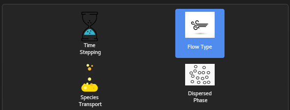
9.2.1 Laminar Flow Model

When the laminar flow option is selected, turbulence closures are disabled and the eddy viscosity is set to zero (). In this regime, viscous transport is governed strictly by molecular dynamic viscosity, making it suitable for low-Reynolds-number flows () or highly viscous fluids while reducing computational cost by omitting additional turbulence transport equations.

9.2.2 GE-RANS Turbulence Model

While many commercial CFD software packages offer an overwhelming array of turbulence models that often cause setup confusion at the user level, NeuralFlow streamlines this selection by incorporating a unified, highly robust approach.

In NeuralFlow, a hybrid formulation is adopted where the – and – turbulence models are combined using a spatial blending function. Under this architecture, the – formulation is activated in the near-wall boundary layer regions to accurately resolve low-Reynolds-number wall effects, whereas the – model is deployed in the freestream domain to eliminate the inherent freestream sensitivity of standard – models. Within both the GUIX-H interface and the core NeuralFlow solver, this blended strategy is formally designated as the GE-RANS (Generalized RANS) turbulence model.

To achieve a unified mathematical structure, an additional cross-diffusion term is introduced into the transport equation for , allowing the – formulation to be transformed directly into an equivalent – representation. Furthermore, this model is strictly coupled with carefully calibrated wall treatments to handle near-wall physical phenomena and manage the primary model transformations reliably.

9.2.3 Scale-Adaptive Simulation (SAS) Model

Scale-Adaptive Simulation (SAS) is a second-generation Unsteady Reynolds-Averaged Navier-Stokes (URANS) formulation designed to bridge the gap between conventional URANS models and Scale-Resolving Simulations such as Large Eddy Simulation (LES). It dynamically adapts the turbulence scale to resolve transient flow structures based on local flow field characteristics and grid resolution.

9.2.3.1 Working Principle and Formulation

The SAS model operates as an advanced variant of the SST – model, where adaptation is achieved primarily through the addition of a dedicated source term () in the transport equation:

URANS Behavior in Stable Regions: Under steady-state conditions or in regions where the spatial grid is too coarse to resolve unsteady fluctuations, the SAS source term remains inactive, causing the model to behave identically to a standard URANS model.
LES-like Behavior in Unsteady Regions: When the flow field exhibits large-scale instabilities and the numerical grid is sufficiently refined, the model detects these fluctuations and dynamically adjusts the turbulent scale, allowing fine-scale, transient eddy structures to be resolved directly.

9.2.3.2 The von Kármán Length Scale

The core mechanism of SAS relies on incorporating the von Kármán length scale () into the transport equation alongside the local strain rate tensor. Unlike traditional URANS models that rely solely on distance-to-wall metrics, the von Kármán length scale is computed using higher-order spatial derivatives of the velocity field:

By accounting for local velocity gradients () and their curvature (), the SAS source term dynamically reduces the modeled turbulent viscosity in unstable flow regimes, enabling the natural development of unsteady, scale-resolved turbulent motion.

9.2.4 Large Eddy Simulation (LES) Model

Caution: Although the Large Eddy Simulation (LES) model is implemented in the solver core and selectable within the GUIX-H interface, it is currently non-functional. Extensive testing and validation are required prior to its operational deployment, and users are strongly advised against using this feature at present.

9.3 Turbulence Model Options

This section details the numerical, physical, and algorithmic options available within the turbulence modeling suite of NeuralFlow. These options control viscous energy dissipation, production limiters, curvature corrections, near-wall formulations, and geometric distance evaluation.

9.3.1 Viscous Dissipation

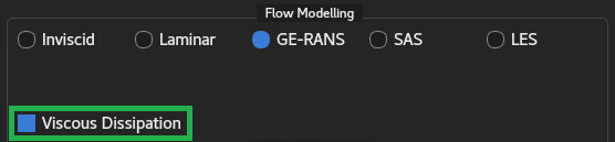
The Viscous Dissipation (also referred to as Viscous Heating) option accounts for the irreversible conversion of kinetic energy into internal thermal energy due to viscous shear stresses. In the total energy conservation equation, this contribution is represented by the viscous work term : While negligible in low-speed incompressible flows (), viscous dissipation becomes critical in high-speed supersonic/hypersonic regimes, narrow channel flows, and highly viscous fluid applications. Enabling this option ensures accurate prediction of aerodynamic recovery temperature, total temperature budgets, and skin-friction-induced thermal loads.

By default, the Viscous Dissipation option is enabled in NeuralFlow to ensure accurate near-wall thermal predictions across all flow regimes. Keeping the Viscous Dissipation model enabled is critical for the accurate evaluation of wall temperatures and surface heat transfer, regardless of whether the domain involves Conjugate Heat Transfer (CHT) or uncoupled fluid boundaries. Within near-wall velocity boundary layers, steep velocity gradients () generate high viscous shear stresses (), converting kinetic energy into localized thermal energy via shear heating (). Neglecting this source term leads to an artificial underestimation of the near-wall fluid temperature and the recovery temperature (). Consequently, this skews the thermal driving potential and wall temperature gradients (), producing inaccurate wall equilibrium temperatures across adiabatic, prescribed heat-flux, and CHT interfaces alike.

9.3.2 GE-RANS Options

The Generalized Eddy-Viscosity RANS (GE-RANS) module offers advanced limiters and structural corrections to enhance stability and accuracy across challenging flow topologies.

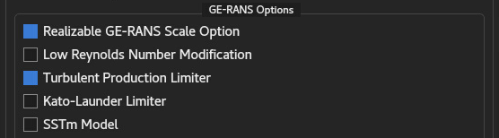
9.3.2.1 Realizable GE-RANS Scale Options

The Realizability constraint enforces mathematical consistency with Reynolds stress physics. Specifically, it prevents unphysical predictions such as negative normal stresses () or violation of the Schwarz inequality () under severe mean strain rates. This is achieved by formulating dynamically rather than treating it as a constant: where is a function of the mean strain and rotation rate tensors. This constraint prevents overprediction of eddy viscosity in regions of extreme velocity gradients, such as boundary layer separation zones and swirling flows.

In regions with extreme mean strain rates and strong velocity gradients (high shear flows, planar/round jets, and swirling boundary layers), enabling the Realizability constraint prevents the unphysical overprediction of turbulent eddy viscosity () and strictly enforces the positivity of normal Reynolds stresses (). Although this dynamic damping of yields superior physical accuracy, the strong non-linear coupling between strain rate invariants and turbulence dissipation can occasionally induce localized numerical oscillations during solver convergence. If convergence fluctuations are observed, using a lower CFL is recommended rather than disabling the option, as maintaining realizability remains strongly recommended for high-shear flow physics.

9.3.2.2 Low Reynolds Number Modification

The Low Reynolds Number Modification introduces damping functions (e.g., ) into the turbulent viscosity and dissipation equations to model viscous sublayer transport directly without relying on algebraic wall functions: As , the damping function ensures that turbulent stresses decay smoothly, allowing molecular viscosity to dominate near solid boundaries. This option requires wall-resolved meshes ().

9.3.2.3 Turbulent Production Limiter

Standard Boussinesq-based RANS models exhibit a well-known non-physical buildup of turbulent kinetic energy in stagnation regions (the stagnation point anomaly) due to high irrotational strain rates . The Turbulent Production Limiter clips the turbulence production term to prevent excessive energy accumulation: This bound stabilizes stagnation point heat flux and drag calculations without compromising shear layer growth downstream.

9.3.2.4 Kato-Launder Limiter

The Kato-Launder Limiter modifies the turbulent production term by replacing the square of the mean strain rate with the product of strain rate magnitude and vorticity magnitude : In stagnation regions where the flow is predominantly irrotational (, ), drops toward zero, effectively eliminating the stagnation point anomaly while preserving standard production behavior in rotational shear layers ().

9.3.2.5 SSTm Model

The Modified Shear Stress Transport (SSTm) model is a tuned variant of the standard SST formulation. While the standard SST model incorporates both strain rate and vorticity invariants in its eddy viscosity limiter, the SSTm variant uses a pure strain-rate-based formulation with modified blending coefficients: SSTm improves numerical convergence in shock–boundary layer interactions, reduces over-conservative separation predictions in mild adverse pressure gradients, and offers enhanced stability for high-speed compressible flows.

9.3.2.6 Curvature Correction

System rotation and streamline curvature significantly alter turbulent shear stress transport. NeuralFlow provides three operational modes for rotation/curvature correction:

Off: Rotation and curvature effects are neglected; production depends strictly on local planar strain rate invariants.
Hellsten: Implements Hellsten’s rotation/curvature correction by scaling the turbulence dissipation/destruction rate equation through a rotational invariant scalar . This enhances turbulence in unstable curved shear layers and suppresses it in rotating vortex cores.
Smirnov-Menter: Employs the Smirnov-Menter formulation, which modifies the turbulent production term using a multiplier based on the Spalart-Shur tensor invariants: where is bounded to provide physical damping in core vortices and enhancement along unstable concave surfaces.

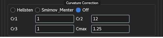
When the Smirnov-Menter curvature correction is selected, the rotation multiplier is governed by four calibration parameters:

(Default = 1.0): Baseline sensitivity factor establishing the linear response of turbulent production to rotation-to-strain rate invariants.
(Default = 12.0): Arctangent scaling parameter controlling the activation growth rate under subtle streamline curvature.
(Default = 1.0): Damping amplitude coefficient governing turbulence suppression strength inside vortex cores.
(Default = 1.25): Absolute upper bound clipping limit on to prevent non-physical turbulence production buildup along unstable concave surfaces.

9.3.2.7 Turbulent Prandtl Number

The Turbulent Prandtl Number () governs the ratio of turbulent momentum diffusivity to turbulent thermal diffusivity:

The default value in NeuralFlow is set to . Decreasing increases turbulent heat conductivity, resulting in higher heat transport rates across turbulent boundary layers. In Conjugate Heat Transfer (CHT) and wall temperature evaluations, directly dictates the thermal boundary layer thickness and wall temperature gradients (), significantly shifting computed surface heat fluxes ().

9.3.3 Wall Treatment

Near-wall formulations bridge the logarithmic layer and viscous sublayer depending on grid resolution.

9.3.3.1 Wall Functions

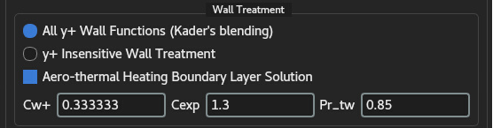
All Wall Functions (Kader’s Blending) [Default]: Utilizes Kader’s exponential blending formulation to provide a smooth, continuous transition between the viscous sublayer () and the fully turbulent logarithmic region (): where is a blending function of . This formulation eliminates numerical discontinuities and ensures -independent solution consistency across arbitrary near-wall grid refinements ( to ).
Insensitive Wall Treatment: Formulated to blend low-Reynolds integration and high-Reynolds wall function boundary conditions automatically, maintaining stable wall shear stress and heat flux predictions regardless of local mesh spacing.

9.3.3.2 Aero-Thermal Heating Boundary Layer Solution

Unlike standard incompressible viscous heating models, the Aero-Thermal Heating Boundary Layer Solution accounts for compressible thermal boundary layer mechanics in supersonic and hypersonic flows (). Near solid boundaries, kinetic energy recovery dictates wall heat transfer via the recovery factor (laminar) or (turbulent): In this formulation, boundary layer heat fluxes are computed relative to the adiabatic wall (recovery) temperature rather than the static freestream temperature, accurately predicting aerodynamic heating and thermal equilibrium in supersonic regimes without impacting subsonic boundary layers.

9.3.4 Wall Distance Method

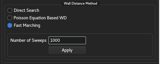
Two-equation models such as SST rely on the minimum distance to the nearest solid boundary () to compute blending functions (), smoothly transitioning from near walls to in the freestream. Three evaluation algorithms are implemented in NeuralFlow:

Direct Search: Computes the exact Euclidean distance from every cell center to all wall faces. While exact, its computational complexity scales as , making it slow for large 3D unstructured meshes.
Poisson Equation Based WD: Solves a Poisson PDE system () to approximate the distance field. Due to numerical diffusion inherent in the Poisson operator, wall distance values away from boundaries tend to be underestimated compared to true geometric distances.
Fast Marching [Default]: An optimized algorithm based on an implicit-tree search structure that solves the Eikonal equation . It delivers exact geometric wall distances with linear computational scaling.

9.3.4.0.1 Recommendation:

It is strongly recommended to keep the Fast Marching method as the active default option. It provides superior numerical accuracy and optimal computational efficiency compared to alternative spatial distance algorithms.