NeuralFlow Theory & User Reference Manual › User's Guide › Getting Started

NeuralFlow User's Guide v2.0 — Chapter 1

1 Getting Started

1.1 Introduction to NeuralFlow

The Compressible Multi-Phase Solver (NeuralFlow) is an advanced multi-dimensional computational fluid dynamics (CFD) code engineered specifically for specialized continuum mechanics and complex multiphase flow topologies. Built upon a rigorous Finite Volume Method (FVM) framework, NeuralFlow utilizes a robust fully-coupled, fully-implicit numerical algorithm capable of executing high-fidelity simulations across 2D planar, 2D axisymmetric, and comprehensive 3D spatial configurations. The solver features native, extensive support for unstructured meshes, including arbitrary polyhedral grids, enabling highly accurate predictive modeling tailored for both demanding industrial deployment and cutting-edge research-level aerospace and fluid engineering workflows.

Engineered for extreme versatility in compressible dynamics, NeuralFlow seamlessly spans an expansive operational envelope that covers fluid behaviors from low subsonic regimes all the way up to high supersonic flow fields. To guarantee seamless user interaction without compromising computational throughput, the architecture relies on a decoupled execution layer characterized by real-time, asynchronous communication with the GUIX-H graphical user interface. This ensures that the frontend remains completely responsive and detached from the underlying heavy linear algebra cycles during stiff multiphase iterations.

1.1.1 Program Capabilities

The Compressible Multi-Phase Solver (NeuralFlow) encompasses a comprehensive suite of cutting-edge numerical features, physical models, and architectural capabilities designed to fulfill the requirements of high-fidelity aerospace and industrial fluid engineering workflows.

1.1.1.0.1 Flow Regimes and Numerical Core

At the core of NeuralFlow is a pressure-based and density-based fully-coupled, fully-implicit algorithm built upon the Finite Volume Method (FVM). By solving the conservation equations for mass, momentum, energy, and phase transport simultaneously within a single matrix system, the solver achieves superior convergence rates and outstanding numerical robustness even when dealing with highly stiff source terms. The spatial discretization schemes are optimized to operate across a remarkably wide velocity spectrum, seamlessly spanning from low subsonic flows up to high supersonic regimes with sharp capturing of compressible effects such as shock waves, contact discontinuities, and expansion fans.

1.1.1.0.2 Mesh and Geometric Flexibility

NeuralFlow offers unrestricted geometric versatility, natively supporting 2D planar, computationally efficient 2D axisymmetric, and full 3D spatial configurations using the exact same underlying solver pipeline. The framework features extensive support for unstructured meshes, including arbitrary polyhedral grids. This polyhedral integration allows the solver to achieve higher spatial accuracy and better gradient calculations with significantly lower cell counts compared to traditional tetrahedral or hexahedral grids, maximizing computational efficiency for complex industrial geometries.

1.1.1.0.3 Advanced Turbulence and Wall Modeling

For turbulent flow regimes, NeuralFlow provides high-performance closures including the Generalized Eddy-Viscosity RANS (GE-RANS) model tailored for severe adverse pressure gradients, the Scale-Adaptive Simulation (SAS) model for unsteady vortex resolving. Crucially, the turbulence framework features advanced -independent momentum and thermal wall functions. These formulations eliminate mesh-density dependence at solid boundaries by automatically blending analytical wall laws with direct numerical resolutions depending on the local grid refinement, ensuring high-fidelity wall shear stress and heat flux predictions independent of .

1.1.1.0.4 Advanced Multiphase Formulations

The solver delivers state-of-the-art multi-fluid Eulerian-Eulerian modeling capabilities augmented by proprietary hyperbolic regularization techniques. These regularizations resolve mathematical singularities typical of pressureless dispersed phases, eliminating artificial diffusion at phase boundaries. Furthermore, dynamic bubble or droplet size tracking is achieved via the integrated One-Group Interfacial Area Transport Equation (IATE). Instead of assuming uniform particle sizes, the dynamic evolution of the interfacial area concentration is mechanistically predicted using advanced sink and source terms for coalescence and break-up driven by turbulence-impact, acceleration-driven (Rayleigh-Taylor), and gravity-driven (Eötvös) mechanisms.

1.1.1.0.5 Thermal Energy and Species Transport

Thermal analysis capabilities include a fully integrated Conjugate Heat Transfer (CHT) model that simultaneously resolves coupled conduction and convection across solid-fluid interfaces. Anisotropic thermal conductivity can be defined as a tensor to accurately capture direction-dependent heat dissipation in advanced composite materials. Additionally, NeuralFlow features native CHEMKIN mechanism ingestion, enabling the automated transport of multi-species chemical components alongside detailed thermochemical production rate tracking.

1.1.1.0.6 Software Architecture, UDF, and Process Automation

Designed for modern engineering infrastructure, NeuralFlow offers unparalleled runtime flexibility. Users can dynamically inject complex physical profiles via transient User-Defined Functions (UDFs) hooked directly into boundary conditions. The UDF capability also allows users to modulate temporal steps as a function of the simulation time in order to actively maintain the physical stability of the simulation. Finally, the multi-process architecture detaches the heavy numerical cycles from the multi-threaded frontend graphical user interface (GUIX-H) via an asynchronous inter-process communication (IPC) loop, ensuring complete UI responsiveness during long cluster runs, while high-level Python bindings (PyNeuralFlow) allow seamless automation for parametric optimization and machine learning integrations.

1.1.2 Known Limitations in NeuralFlow and GUIX-H (v2.0)

While NeuralFlow v2.0 introduces powerful multiphase and compressible flow modeling capabilities, users must account for the following algorithmic, physical, and architectural constraints during simulation design and computational resource allocation:

Computational Cost per Iteration: Owing to the fully-coupled, fully-implicit formulation of the numerical core, the CPU wall-clock time required to complete a single iteration is higher than that of traditional segregated solvers. However, because the implicit coupling dramatically improves matrix stability and permits much larger time steps, the overall total time-to-convergence remains of a comparable order of magnitude due to a significantly reduced total iteration count.
High Memory (RAM) Footprint: The simultaneous solution of mass, momentum, energy, and phase transport equations within a single, unified linear system inherently demands a high random-access memory (RAM) allocation per cell. Users must ensure adequate hardware memory configurations, particularly when deploying large-scale unstructured or polyhedral grids.
Incompatibility with Binary Mesh Formats: The grid ingestion pipeline is strictly limited to ASCII-encoded file formats. NeuralFlow v2.0 cannot parse or interpret binary-formatted mesh (.msh) files generated by ANSYS Meshing or ANSYS Fluent. Consequently, users must ensure that computational grids are explicitly exported or converted into the standard ASCII text format during the pre-processing phase before attempting mesh ingestion.
Absence of Adaptive Mesh Refinement: Adaptive Mesh Refinement (AMR) features are entirely absent in the current release. The solver does not support dynamic mesh optimization, isotropic cell splitting, or automated localized refinement during runtime for any grid topology.
Non-Functional LES Solver: The Large Eddy Simulation (LES) solver module is currently non-functional and disabled in this version. Core development efforts to address, optimize, and re-enable these filtered subgrid-scale turbulence models are strictly planned for future software updates.
Unvalidated Multiple Reference Frame (MRF): The Multiple Reference Frame (MRF) functionality for rotating domains has not yet undergone comprehensive testing and verification. Consequently, its deployment in production-grade or research-level rotating frame simulations is not recommended at this stage.
CGNS Interoperability and Implementation Discrepancies: Although the CFD General Notation System (CGNS) is conceptually architected as a universal, platform-independent standard, in practice, various commercial and open-source software vendors adopt diverging implementation conventions regarding the underlying Standard Interface Data Structures (SIDS). Due to these distinct file-structure variations across the industry, seamless cross-platform compatibility is frequently compromised. NeuralFlow v2.0 is subject to this limitation; the internal CGNS reader expects a strict topological and boundary-state layout mapping, meaning that CGNS files exported from certain external preprocessing or simulation toolchains may fail to parse correctly or result in ingestion errors.
Platform Compatibility and Operating System Constraints: Currently, the GUIX-H graphical interface, the NeuralFlow solver core, and all associated third-party dependency libraries are compiled and linked exclusively for the CentOS 7 operating system environment. Deployment workflows, cross-compilation pipelines, and native binary packages for alternative Linux distributions or other operating systems are not yet mature. Consequently, attempting to execute the software suite on unsupported platforms may result in critical dynamic linking failures, library mismatches, or unstable runtime behaviors.
Untested Process Launchers and Workload Managers: Within the Solvers configuration interface, the customizable Launcher settings and Workload Manager backend options designed for spawning and scheduling NeuralFlow processes remain unvalidated and have not undergone comprehensive verification. To prevent process initialization failures and ensure stable execution, both parameters are strictly restricted to their default "Auto" setting. Users are strongly discouraged from selecting alternative manual configurations in this release, as they may disrupt the process spawning sequence or corrupt the communication handshake.

1.1.3 Supported Third-Party Software and Libraries

To achieve high performance, exact numerical differentiation, and seamless data interoperability, NeuralFlow integrates a robust ecosystem of industry-standard third-party libraries and file formats. These dependencies are leveraged across pre-processing, core linear algebra acceleration, parallel execution, and post-processing stages:

1.1.3.0.1 Pre-Processing and Mesh Interoperability

Supported Meshing Files: NeuralFlow natively parses external .msh (ASCII format only) grid files generated and exported by ANSYS computational preprocessing toolchains, mapping standard zone definitions directly into the internal Finite Volume framework. The same ASCII .msh format exported by other tools that ANSYS Fluent supports can also be used. Standardized CGNS grid exported by any meshing tool can also be imported to NeuralFlow.
ANSYS Fluent Material Database (.scm): The solver supports the direct ingestion of Fluent-compatible scheme-formatted (.scm) material databases, automating the allocation of thermodynamic and transport properties.Additionally, NeuralFlow natively supports its own custom material database format structured in JSON (JavaScript Object Notation). This format provides a lightweight, human-readable, and highly structured schema, making it exceptionally easy to inspect, edit, or generate programmatically using external scripts.(.mdb) in JSON format.
CGNS (CFD General Notation System): Supported as a standardized, platform-independent file format for the efficient storage, exchange, and retrieval of multi-zone CFD grid topologies and solution data across different computational platforms.

1.1.3.0.2 Core Mathematical Solvers and Differentiation

PETSc (Portable, Extensible Toolkit for Scientific Computation): Outlines the scalable linear solver backbone of NeuralFlow. It supplies the parallel Krylov subspace solvers (e.g., GMRES, BiCGStab) and advanced preconditioning options necessary for driving the fully-implicit coupled algorithms.
Intel MKL (Math Kernel Library): Utilized for low-level vectorization and kernel-level mathematical operations. Intel MKL optimizes heavy matrix-vector products and basic linear algebra subprograms for processor architectures.
CoDiPack (Code for Differentiation Package): Integrated to provide high-performance forward-mode Automatic Differentiation (AD). CoDiPack computes exact, algorithmic Jacobians required by the stiff fully-coupled implicit solver loop, avoiding the precision losses of finite-difference approximations.

1.1.3.0.3 Graph Partitioning and Multigrid Acceleration

METIS: A serial graph partitioning library used during the pre-execution phase to divide arbitrary unstructured and polyhedral meshes into highly optimized, well-balanced subdomains, minimizing the surface-to-volume ratio across parallel zones.
MGridgen: Acts as the underlying topological engine for the Geometric Multigrid (GMG) sequence, generating coarser mesh representations via cell agglomeration to accelerate low-frequency error dissipation in linear systems.

1.1.3.0.4 Parallelism, IPC, and Software Automation

MPICH: Serves as the message-passing framework responsible for message-passing interface (MPI) execution across distributed-memory high-performance computing clusters. Additionally, MPICH is leveraged to manage low-latency asynchronous inter-process communication (IPC) between the core computation backend (NeuralFlow) and the frontend interface (GUIX-H).
Python 3.11: Embeds a runtime Python interpreter to empower the high-level PyNeuralFlow scripting pipeline and execute automated parametric sweeps, while facilitating dynamic runtime parsing for advanced User-Defined Functions (UDFs).
Boost: Provides foundational C++ standard utility extensions, cross-platform file system abstractions, and advanced data structures ensuring robust structural memory safety within the core software architecture.

1.1.3.0.5 Post-Processing and Data Visualization

VTK Toolkit (Visualization Toolkit): Handles advanced solution field extraction and data encapsulation. NeuralFlow relies on VTK APIs to write parallel unstructured XML data sheets (.vtu), allowing immediate post-processing and volumetric visualization within tools like ParaView.

1.2 Basic Steps for CFD Analysis using NeuralFlow

The operational pipeline for executing a simulation within the NeuralFlow framework follows a structured sequence of engineering and numerical tasks:

Define the Modeling Goals: Clearly identify the primary physical phenomena of interest and determine the required quantitative engineering outputs of the simulation.
Generate and Simplify Geometry: Create the computational fluid domain and remove non-essential geometric features to minimize topological complexity and enhance mesh generation quality.
Discretize the Computational Domain: Construct a high-quality mesh, ensuring sufficient cell clustering and proper wall spacing within near-wall boundary layers.
Initialize the Execution Interface: Launch the GUIX-H graphical user interface (if PyNeuralFlow script is not used) to establish an asynchronous communication link and spawn the active backend NeuralFlow solver process.
Configure Physical and Continuum States: Select the appropriate models, define material characteristics for all cell zones, and prescribe exact boundary condition states.
Set Up Monitoring and Data Operations: Define runtime surface or point monitors, configure report metrics, and establish automated intervals for saving solution and VTU data.
Compute the Solution: Initialize the flow field state vectors and initiate the solver loop to advance the system toward steady or transient numerical convergence.
Examine and Export Results: Review the converged data using localized visualization tools or external post-processors, and securely write the final solution data files.
Evaluate and Refine Models: Assess the physical and mathematical validity of the converged state, and implement necessary revisions to the mesh topology, boundary variables, or numerical schemes if discrepancies arise.

Important Note: To prevent irreversible data loss in the event of numerical divergence during highly coupled iterations, users are strongly advised to configure appropriate autosave frequencies for intermediate solution files, ensuring that computational progress can be recovered efficiently without restarting the simulation from the initial state.

1.3 Starting and Executing NeuralFlow

1.3.1 Starting NeuralFlow with GUIX-H

When executing simulations within the graphical ecosystem, the software architecture establishes a strict process hierarchy where the graphical user interface (GUIX-H) acts as the master supervisor layer positioned directly above the computational backend solver (NeuralFlow). A core advantage of this decoupled architecture is its multi-solver management capability, allowing a single, active GUIX-H instance to concurrently oversee and communicate with multiple independent NeuralFlow processes. Therefore, to initiate a solver, the user must first launch the GUIX-H application. The interface then serves as the primary orchestration hub responsible for spawning individual, decentralized NeuralFlow backend solver processes. To launch GUIX-H, execute the following command in your shell at the directory where it is deployed:

$ ./run_guix

1.3.1.1 Setting Working Directory in NeuralFlow Launcher

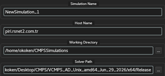
Working directory for autosave options and User-Defined Functions (UDFs) could be defined under the Solvers tab; and solver is spawned under the Working Directory with the defined Simulation Name.

Layout of Simulation Name and Working Directory

1.3.1.2 Setting Dimension in NeuralFlow Launcher

During the solver spawning phase within the GUIX-H solver configuration panel, the user must explicitly define the spatial dimensionality of the target simulation. Depending on the dimension selected by the user, the GUIX-H supervisor layer dynamically invokes the specific native executable required for the task; 2D and 3D.

Note: The dimensionality parameter must strictly match the spatial layout of the imported mesh file. Once a NeuralFlow solver instance is spawned, its dimension mode is structurally immutable; changing from a 2D to a 3D setup or vice-versa requires terminating the active backend process and initializing a new solver instance with the appropriate grid-compatible binary.

1.3.1.3 Setting Parallel Options in NeuralFlow Launcher

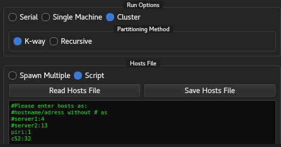
Within the GUIX-H Launcher panel, users can configure shared or distributed memory options by selecting the Run Options radio button, and then defining the number of MPI processes, and linking to the specific hosts allocation map.

Under the Run Options panel, the interface exposes three distinct execution modes to suit different hardware environments:

Serial: Spawns a single-processor (1-CPU) NeuralFlow solver instance on the local master machine. This mode bypasses parallel orchestration overhead entirely and is suitable for simple mesh diagnostics, localized 2D test verifications, or low-fidelity preprocessing tasks.
Single Machine: Initiates an -processor parallel NeuralFlow solver instance on the local master machine. This option leverages shared-memory multi-core architectures on a single system to scale the numerical computation locally, utilizing the specified processor count .
Cluster: Enables distributed-memory parallel execution across multiple interconnected computer nodes. In this mode, the user must explicitly define the computational hostnames and their corresponding processor allocations. This configuration employs a hybrid parallelization strategy—utilizing high-speed shared-memory mechanisms within the same physical machine and distributed-memory message passing (MPI) across distinct machines—to run a unified, highly-scaled NeuralFlow solver process.

Layout of Parallel and Partitioning Options

Important Architectural Considerations:

Master-Worker Orchestration: When utilizing either the Single Machine or Cluster parallel configurations, one processor is automatically assigned as the main node (master process). This dedicated node does not participate directly in the local stencil computations; instead, its primary role is to orchestrate workload distribution among the remaining worker nodes and manage all bidirectional control and data communication with the master GUIX-H interface.
Cluster Master Resource Allocation: If the Cluster option is selected, the main (orchestration) node should ideally be assigned to a master machine equipped with high memory capacity (RAM). This ensures that global data aggregation, convergence checks, and GUI state updates are handled efficiently without memory bottlenecks, as illustrated schematically in Figure 1.3.

Once the target parallel processor count is established, the computational grid must be decomposed (partitioned) among the allocated MPI ranks to balance the numerical workload and minimize inter-process communication latency. To achieve high-efficiency domain decomposition, NeuralFlow integrates the industry-standard METIS graph partitioning library. Within the launcher interface, users can select between two distinct partitioning algorithms based on their computational scale:

K-Way Partitioning (Default Option): This algorithm utilizes a multilevel paradigm to partition the mesh graph directly into the target subdomains in a single, globally-optimized operational sweep.
- Advantages: Highly computationally efficient with rapid execution times, making it the ideal choice for large-scale meshes and high-performance computing (HPC) environments with high core counts (typically ). Because it evaluates the entire domain globally, it minimizes the total edge-cut (the interface boundaries between processors), which drastically reduces the MPI communication bottleneck during tightly-coupled implicit solver iterations.
- Disadvantages: On highly irregular or hybrid unstructured topologies, it may exhibit slightly relaxed cell-count balancing tolerances compared to recursive methods.
Recursive Partitioning: This approach recursively bisects the mesh graph into two halves, repeating this binary split sequence until the exact number of desired partitions is achieved.
- Advantages: Offers superior and aggressive load-balancing metrics. It ensures that the cell count distributed to each processor is virtually identical, which is highly beneficial for lower core counts (specifically powers of two, such as or cores) and simpler mesh topologies.
- Disadvantages: The computational overhead of the partitioning phase scales log-arithmetically and becomes significantly slow as the target partition count grows. Additionally, due to its localized binary-split decisions, it can suffer from "global blindness," potentially yielding a higher total edge-cut and increased MPI messaging overhead in massive parallel runs.

User Recommendation: For localized desktop simulations running on low core counts (), Recursive Bisection is recommended to ensure tight load balancing. For large-scale multi-node cluster deployments utilizing modern HPC resources ( cores), users should explicitly select K-Way partitioning to minimize pre-processing times and eliminate inter-node communication bottlenecks.

1.3.2 Starting NeuralFlow with PyNeuralFlow

!!! WILL BE UPDATED !!! PyNeuralFlow provides a high-level scripting entry-point using Python bindings for optimized automation.

import pyneuralflow
session = pyneuralflow.Launcher(mode="headless")

1.3.2.1 Setting Parallel Options in PyNeuralFlow Launcher

Parallel configurations can be explicitly stated within the initialization parameters:

session.set_parallel(cores=16, backend="openmpi")