10 Modeling Thermal Energy
10.1 Introduction
Heat transfer describes the exchange of thermal energy across space resulting from temperature gradients between different physical regions or media. Thermal energy transport fundamentally occurs via three primary mechanisms: conduction, convection, and thermal radiation.
Depending on the physical complexity of the application, thermal simulations in NeuralFlow encompass Conduction and Forced Convection operational regimes.
Note on Radiation Modeling:
Currently, NeuralFlow does not support full radiation models such as Discrete Ordinates (DO) or Surface-to-Surface (S2S). However, radiative thermal effects can still be accounted for at domain boundaries by specifying external radiation within the wall thermal boundary condition settings.
When thermal effects are enabled, NeuralFlow automatically solves a tailored formulation of the energy conservation equation that incorporates the specific heat transfer mechanisms activated by the user. Furthermore, for domain configurations with spatial repetition, periodic heat transfer boundary conditions can be utilized to substantially lower cell counts and reduce overall computational cost.
10.2 Modeling Conjugate Heat Transfer
Solves coupled conduction and convection problems at solid and fluid domains simultaneously. In high-speed and high-enthalpy flow regimes, a significant time scale disparity exists between fluid dynamic phenomena and solid thermal conduction; the characteristic time scale of the fluid is typically orders of magnitude smaller than the thermal diffusion time scale within the solid domain. Advancing the entire coupled domain uniformly using the small time step size dictated by the fluid physics leads to excessive computational overhead and prolonged simulation turnaround times.
To mitigate this computational bottleneck, NeuralFlow decouples the execution frequencies of the fluid and solid solvers in Conjugate Heat Transfer (CHT) simulations:
Solid Domain: Pure thermal conduction within solid regions is resolved at every physical time step, maintaining continuous temporal tracking of heat diffusion.
Fluid Domain: The full system of fluid flow equations and active physical models are evaluated at a user-defined interval (solving frequency) rather than at every single time step.
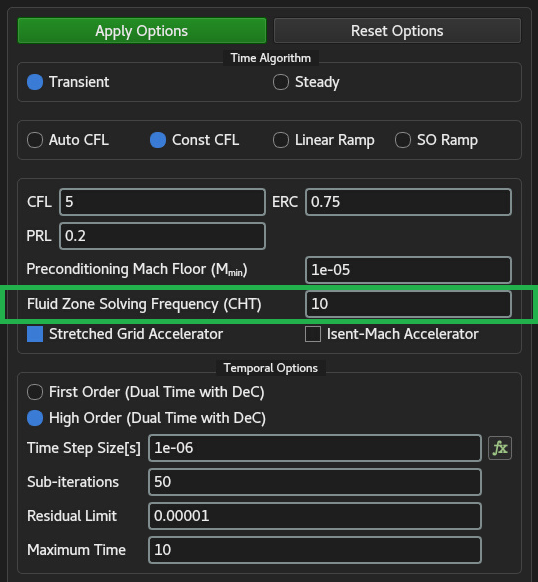
By periodically solving the fluid domain, the thermal boundary layer and interfacial heat flux distributions are refreshed dynamically. This dual-frequency approach ensures accurate temperature predictions across the fluid-solid interface while dramatically accelerating overall solution efficiency.
10.3 Supported Wall Thermal Boundary Conditions
At flow inlets and exits you will set the temperature; at walls you may use any of the following thermal conditions:
Adiabatic
Specified heat flux
Specified temperature
Convective heat transfer
External radiation
Combined external radiation and external convective heat transfer
10.4 Solution Strategies for Heat Transfer Modeling
10.4.1 Transient Solid Heat Conduction
For transient solid heat conduction simulations in NeuralFlow, the following key physical and numerical aspects apply:
Governing Equation: Within pure solid zones, NeuralFlow solves the unsteady heat conduction equation, accounting for transient energy storage, spatial thermal diffusion, and volumetric heat generation:
where is density, is specific heat capacity, is thermal conductivity, and is the volumetric heat generation rate. Material Properties: Unlike steady-state conduction (which depends solely on thermal conductivity
), transient thermal response is dictated by thermal diffusivity ( ). Therefore, accurate values for density ( ), specific heat capacity ( ), and thermal conductivity ( ) must be defined. Temporal Discretization: The transient formulation utilizes a fully implicit time-integration scheme based on dual time-stepping, ensuring numerical stability even when using larger time steps relative to thermal diffusion scales.
Initial Conditions: A physically realistic initial temperature field across the solid domain is required to establish accurate time-dependent thermal histories.
Interface Thermal Coupling: At solid-solid contact regions, continuous heat flux and temperature matching are enforced automatically to model thermal boundary layer dynamics and conjugate heat transfer.
Note on Computational Efficiency:
The employment of an implicit dual-time stepping scheme enables the use of significantly larger physical time step sizes without compromising numerical accuracy. Consequently, transient thermal simulations can be completed with substantially reduced overall execution times.
Note on Fluid Zone Solving Frequency:
In pure transient solid heat conduction simulations where no fluid domain exists, the value specified for Fluid Zone Solving Frequency within the Solution Control Tool has no effect on the simulation.
10.4.2 Transient Conjugate Heat Transfer
Transient Conjugate Heat Transfer (CHT) models the coupled, time-dependent thermal energy exchange between fluid flows and solid structures. Unlike uncoupled thermal simulations where wall temperatures or heat flux values are prescribed statically, transient CHT simultaneously resolves convective and conductive energy transport in the fluid domain alongside thermal diffusion within adjacent solid regions, continuously updating the thermal state across shared interfaces.
At the fluid-solid boundary, physical coupling requires that both temperature continuity and flux conservation are strictly satisfied at every active coupling step:
The fundamental challenge in transient CHT arises from the severe
disparity in physical time scales between the fluid and solid domains.
Fluid flow transport is typically dictated by fast convective and
turbulent time scales, whereas solid thermal propagation is governed by
thermal diffusivity (
When configuring transient CHT simulations in NeuralFlow, the following key operational and physical aspects should be highlighted:
Interfacial Thermal Response: The accurate capture of transient temperature gradients inside the solid depends directly on the volumetric heat capacity (
) of the solid material and the local convective heat transfer coefficient provided by the fluid boundary layer. -Independent Wall Functions: The momentum and thermal wall functions in NeuralFlow are formulated to be -independent. Consequently, thermal boundary layer predictions and wall heat flux calculations demonstrate minimal sensitivity to near-wall cell height, relaxing grid refinement constraints and removing the strict requirement for . Time-Stepping Strategy: Utilizing implicit time-integration along with dual-time stepping allows the solver to maintain numerical stability and high solution accuracy across varying physical time scales.
Computational Efficiency via Multi-Frequency Coupling: By combining multi-frequency fluid solving with sub-iterative interfacial coupling, users can bypass unnecessary fluid transport calculations during slow solid heat soaking periods, drastically accelerating total runtimes.
Typical application areas for transient CHT in NeuralFlow include aerodynamic heating on high-speed airframe structures, thermal shock analysis in engine nozzles and turbine blades, and startup/shutdown thermal transients in electronic cooling systems.
Transient Conjugate Heat Transfer (CHT) concurrently resolves conductive energy transport within solid domains and convective flow dynamics in adjacent fluid regions. In high-speed and high-enthalpy flow regimes, a pronounced disparity exists between the rapid time scales of fluid dynamic phenomena and the much slower thermal diffusion process within solid structures. Uniformly advancing the entire coupled domain using the small time step size dictated by the fluid physics introduces severe computational overhead and unnecessarily prolonged turnaround times.
To overcome this computational bottleneck, NeuralFlow incorporates a multi-frequency solver architecture for CHT simulations:
Solid Domain: Unsteady thermal conduction inside solid zones is computed at every physical time step, maintaining continuous temporal tracking of thermal diffusion.
Fluid Domain: The full system of fluid flow equations and active physical models is evaluated at a user-defined interval (Fluid Zone Solving Frequency) rather than at every single time step.
By periodically updating the fluid flow field, the thermal boundary layer and interfacial heat flux distributions are refreshed dynamically. This dual-frequency approach maintains accurate interfacial temperature predictions while dramatically accelerating overall solution efficiency.
Recommendation on Time Stepping & Solving Frequency:
During the initial transient phase, where rapid thermal gradients and high heat flux rates dominate, it is recommended to utilize a smaller time step size accompanied by a low Fluid Zone Solving Frequency (approximately 1). As the local thermal gradients relax and heat flux rates stabilize, both the time step size and the Fluid Zone Solving Frequency can be progressively increased (typically to a range of 10–50) to maximize computational efficiency without compromising solution accuracy.