11 Modeling Dispersed-Phase
11.1 Eulerian Dispersed-Phase Governing Equations
In NeuralFlow, the dispersed particle or droplet phase is formulated as a
continuum using a compressible Eulerian framework. The conservative
transport state of the dispersed phase is represented by the mass
concentration
The governing hyperbolic conservation laws with regularized stress
tensors and dynamic interfacial transport are written in compact system
form as:
11.1.1 Hyperbolic Regularization for Pressureless Dispersed Systems
Standard dilute Eulerian formulations lack an intrinsic thermodynamic
pressure gradient, causing characteristic wave speeds to collapse to
local particle velocity (
To eliminate these mathematical singularities while preserving true
pressureless transport in dilute zones, NeuralFlow incorporates a
velocity-gated friction pressure law:
11.1.2 Receiver-Side Packing Flux Limiter
To enforce the maximum physical packing limit
—
11.2 Dispersed Phase Options
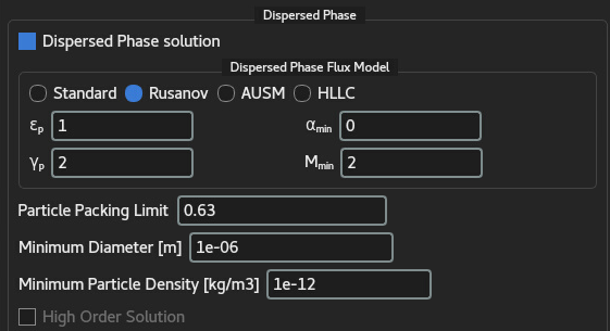
The Dispersed Phase module NeuralFlow governs multi-phase flow interactions using a Eulerian-Eulerian formulation. This approach treats the dispersed particulate, droplet, or liquid droplet cloud as a continuous phase coexisting with the continuous gas phase.
11.2.1 Dispersed Phase Solution Activation
Dispersed Phase Solution [Checkbox]: Enables or disables the transport and conservation equations for the dispersed phase (mass, momentum, thermal energy, and optional interfacial area concentration). When disabled, the solver operates strictly in single-phase mode.
11.2.2 Dispersed Phase Flux Model
Pressureless Eulerian formulations for dispersed phases inherently suffer from mathematical ill-posedness (loss of hyperbolicity) and singular density concentrations (delta-shocks) during particle trajectory crossing or deceleration. To evaluate numerical fluxes across cell faces, NeuralFlow provides four distinct Riemann flux formulations:
Standard: A baseline upwind/central flux formulation for degenerate system. The upwinding-based dispersed phase flux method referred to as Standard is intended for degenerate, i.e., weakly hyperbolic systems. Its use is strictly not recommended.
Rusanov: A Lax-Friedrichs type Riemann solver that uses the maximal local spectral wave speed (
) to scale numerical dissipation. It provides exceptional stability and robustly smooths out singular particle density spikes in complex shock-particle interactions. AUSM (Advection Upwind Splitting Method): Separates convective and pressure-like regularization flux components. AUSM preserves sharp particle volume fraction gradients without excessive numerical diffusion along phase contact surfaces.
HLLC: A three-wave Harten-Lax-van Leer Riemann solver with explicit contact wave restoration. It delivers high physical resolution for isolated particle fronts, boundary layer shear layers, and expanding droplet plumes.
11.2.3 Hyperbolic Regularization Parameters
To eliminate singularity issues in pressureless dispersed phase
formulations, an artificial hyperbolic regularization pressure (
(Artificial Pressure Coefficient) : Scales the overall magnitude of the hyperbolic regularization pressure term. Increasing adds numerical stability near extreme deceleration zones at the expense of artificial particle dispersion. (Regularization Exponent) : Defines the polytropic index governing the non-linear growth of regularization pressure with respect to local particle concentration. A value of provides quadratic resistance against non-physical particle packing. (Volume Fraction Floor) : Sets the absolute minimum threshold for dispersed phase volume fraction ( ). Prevents zero-density mathematical evaluation errors in pure gas regions. (Preconditioning/Spectral Floor) : Establishes the minimum pseudo-Mach bound used within the flux Jacobians to stabilize signal propagation speeds when local particle velocity approaches zero ( ) near stagnant regions.
11.2.4 Physical Limits and Numerical Bounding
Particle Packing Limit : Defines the maximum physically allowable volumetric packing ratio (
) for solid particles (corresponding to random close packing of rigid spheres ). When local reaches this limit, granular pressure forces rise steeply to prevent inter-particle overlap and unphysical volume fraction values ( ). Minimum Diameter [m] : Sets the lower physical bound for mean particle/droplet diameter (
). Protects drag law correlations (e.g., Schiller-Naumann or Clift) from division-by-zero singularities ( ) during breakup or evaporation processes. It is used only when dynamic size tracking (IATE) is active. Otherwise, particle size remains constant as it is defined in Materials Tool. Minimum Particle Density [kg/m
] : Establishes the minimum mass concentration floor for the dispersed phase. Ensures matrix non-singularity in computational cells void of particles while maintaining strict conservativeness. High Order Solution [Checkbox]: Controls the spatial discretization accuracy of the dispersed phase transport equations. When disabled (OFF), a robust first-order upwind scheme is used. When enabled (ON), higher-order reconstruction with flux limiters is applied, preserving sharp spatial gradients and preventing numerical smearing of droplet spray boundaries. Currently, it is disabled for all cases since it requires more testing.
11.3 Boundary Conditions for Dispersed-Phase Transport
Proper boundary specification closes the continuous-dispersed continuum equations:
Inlets: Users prescribe the inlet mass concentration
(or volume fraction ), temperature , and velocity vector . If velocity slip is assumed at entry, interphase drag accelerates particles toward continuous-phase velocity. Outlets: Zero-gradient Neumann conditions (
) are applied to conserved variables at supersonic or pressure outlet boundaries. Solid Walls: Solid boundaries enforce either no-slip (
) or free-slip ( ) conditions based on surface wall-function configurations, while normal mass fluxes satisfy zero net penetration ( ).
11.4 Dynamic Size Tracking via One-Group IATE
To capture particle breakup and coalescence without the prohibitive
computational cost of full population balance models, NeuralFlow tracks the
evolution of the interfacial area concentration
The local Sauter mean diameter
The transport equation for one-group interfacial area concentration
is given by:
11.4.1 Coalescence and Breakup Source Terms
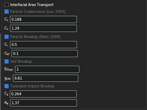
All source terms in NeuralFlow are constructed using
Random Turbulence Coalescence (
): Models inter-particle collisions driven by continuous-phase turbulent fluctuations ( ). Breakup Mechanisms (
): Encompasses dynamic process sources that generate interfacial area density by fragmenting particles through fluid dynamic forces: Acceleration-Driven Breakup (
): Induced by Rayleigh–Taylor instabilities when the interface undergoes strong relative acceleration, rapidly growing surface perturbations that fragment the particle. It can be described as a function of particle slip velocity. Turbulence-Impact Shattering (
): Occurs when energetic continuous-phase turbulent eddies collide with particles; if the turbulent kinetic energy exceeds the surface tension energy barrier, the particle shatters. A reduction in droplet size intensifies turbulent breakdown. Gravity-Driven Breakup (
): Dictated by Eötvös-type forces that establish the maximum stable particle size ( ), where buoyancy forces dominate surface tension beyond critical thresholds ( ), driving interface distortion, elongation, and pinch-off.
11.4.2 Boundary Conditions for Interfacial Area Concentration
Inlets: Users specify the initial particle diameter (
), dispersed phase mass fraction ( ), and particle temperature ( ) at inlet boundaries. Although the mass fraction and particle temperature are standard inputs required for the base dispersed phase transport equations regardless of whether the IATE model is active, the initial particle diameter is explicitly used to compute the inlet interfacial area concentration ( ) via: where is the effective density of the dispersed phase at the inlet and is the phase material density evaluated at the specified inlet particle temperature. Outlets and Walls: Zero-gradient conditions (
) are applied across non-reacting wall and outflow boundaries.