7 Solver Options
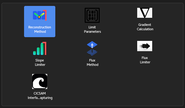
This chapter details the spatial discretization, flux reconstruction, and numerical control options available in the solver. Choosing appropriate reconstruction schemes is critical for balancing numerical stability, spatial accuracy, and non-physical dissipation. The whole options related to solver can be reached from Numerics Tool.
7.1 Reconstruction Methods
Reconstruction methods govern how cell-centered flow quantities
(
7.1.1 First Order Scheme
Numerical Formulation: Reconstructs the cell-face value using a piecewise constant approximation based strictly on the upwind cell-center value:
where represents the quantity in the cell immediately upwind of the face. Local variable gradients are completely neglected during face reconstruction. Characteristics: Unconditionally stable, robust, and strictly monotonic. However, it introduces significant numerical diffusion (false dissipation), which artificially smears steep boundary layers, shock waves, and shear stress gradients (
-order spatial accuracy). Recommended Usage: Ideal for initial solution startup to establish a baseline flow field, or for highly unstable shock-dominated initializations.
7.1.2 Second Order Scheme
Numerical Formulation: Reconstructs face quantities via piecewise linear extrapolation by combining the upwind cell-center value with local cell gradients:
where is the local spatial gradient of the upwind cell and is the displacement vector from the upwind cell centroid to the face centroid. Slope limiters are applied to preserve solution monotonicity. Characteristics: Delivers
-order spatial accuracy with dramatically reduced numerical dissipation. Accurately resolves boundary layer profiles, aerodynamic forces, and vortex structures. Recommended Usage: Default baseline configuration for general steady-state and time-accurate production CFD simulations.
7.1.3 Bounded Central Differencing (BCD)
Note. Verification Status Warning: The Bounded Central Differencing (BCD) reconstruction method is currently undergoing active numerical verification and validation. Users should exercise caution when interpreting fine-scale unsteady results until validation routines are fully concluded.
Numerical Formulation: Blends non-dissipative
-order central differencing ( ) with a stable upwind scheme ( ) using a flux limiter based on the Normalized Variable Formulation (NVF): where is the local blending factor determined dynamically by local solution bounds and the user-defined threshold. Characteristics: Minimizes numerical dispersion and artificial damping, allowing transient turbulent eddies and acoustic waves to propagate without numerical attenuation while preventing non-physical oscillations.
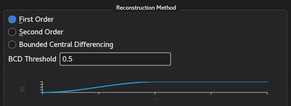
Reconstruction Parameters - BCD Threshold: Defines the blending criterion threshold (
) for the non-linear NVF limiter (default: ). Lower values increase first order upwind blending for enhanced solver stability, whereas higher values enforce central differencing for low-dispersion vortex resolution. Recommended Usage: Intended for scale-resolving unsteady flow simulations, such as Large Eddy Simulation (LES) and Scale Adaptive Simulation (SAS) / Detached Eddy Simulation (DES).
7.2 Limiting Parameters
During the non-linear iterative solution procedure—particularly during initial startup phases or high-gradient transient impulses—unbounded numerical updates can lead to unphysical variable values (e.g., negative temperatures, near-zero absolute pressures, or runaway turbulence levels). The Limit Parameters panel enforces hard numerical bounds (clamping thresholds) on key flow variables. These bounds stabilize the linear matrix solvers without altering converged physical steady-state solutions.
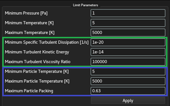
The set of active limit parameters dynamically adapts based on the active physics models enabled in the simulation (e.g., turbulence closures, compressible energy equations, and dispersed multiphase models).
7.2.1 Thermodynamic Property Limits
Global thermodynamic bounds apply to the primary fluid phase to maintain physical state-variable boundaries:
Minimum Pressure [Pa]: Sets an absolute lower bound on local static pressure (default:
). This prevents non-physical negative pressures or vacuum singularities in strong expansion waves or shock-capturing routines. Minimum Temperature [K]: Enforces an absolute lower bound on fluid static temperature (default:
), preventing numerical underflow and thermodynamic state-variable divergence in cold expansion regions. Maximum Temperature [K]: Caps the upper bound of static fluid temperature (default:
) to prevent unphysical localized temperature spikes caused by transient energy flux overshoots.
7.2.2 Turbulence Model Limits
When a two-equation turbulence model (such as
Minimum Specific Turbulent Dissipation [1/s]: Specifies the lower limit for the specific dissipation rate (
, default: ). Enforcing a non-zero lower floor prevents division-by-zero singularities when computing eddy viscosity . Minimum Turbulent Kinetic Energy [m
/s ]: Clamps the minimum allowable value for turbulent kinetic energy ( , default: ) to ensure positive-definiteness of the turbulent transport matrix. Maximum Turbulent Viscosity Ratio [-]: Caps the maximum ratio of turbulent dynamic viscosity to molecular dynamic viscosity (
, default: ). This suppresses unphysical, runaway turbulence production during early solution iterations.
7.2.3 Dispersed-Phase Limits
When Eulerian multiphase or dispersed-phase particle transport models are activated, additional bounds are enforced to regulate the dispersed phase physics:
Minimum Particle Temperature [K]: Sets the absolute lower temperature threshold for the dispersed particle/droplet phase (default:
). Maximum Particle Temperature [K]: Sets the upper temperature ceiling for the dispersed phase (default:
) to bound phase-change and interphase heat transfer computations. Maximum Particle Packing [-]: Defines the maximum allowable volume fraction limit (
) for close-packed solid particles or droplets (default: ). This reflects the maximum random close-packing limit of spherical particles, preventing non-physical volume fraction accumulation in concentrated multiphase transport equations.
7.2.4 Applying Limit Modifications
Modifications to any bounding limits are updated in solver memory by clicking the Apply button at the bottom of the control panel.
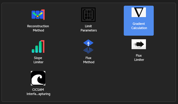
7.3 Gradient Calculation
Accurate computation of cell-centered spatial gradients (

7.3.1 Green-Gauss Method
Mathematical Formulation: Applies Gauss’s divergence theorem over the control volume
by converting the volume integral of the gradient into a summation of variable values over cell faces: where is the outward-pointing face area vector and is the face-centered variable value, typically approximated via arithmetic weighting of adjacent cell centroids. Pros: Low computational cost and minimal memory overhead. Highly accurate on structured, orthogonal, or mildly skewed hexahedral meshes.
Cons: Highly sensitive to mesh non-orthogonality, cell aspect ratio, and grid skewness. On distorted unstructured grids, face-value interpolation errors can degrade gradient accuracy and trigger spurious numerical oscillations.
Recommended Usage: Ideal for high-quality structured/multiblock meshes or simple geometric domain configurations.
7.3.2 Least Squares Method
Mathematical Formulation: Assumes a linear variation of the field variable between cell centroids. The gradient vector
is determined by minimizing the weighted sum of squared errors across all immediate face-sharing neighbor cells ( ): where is the displacement vector connecting the owner cell centroid to neighbor centroids, and is a distance-based weighting factor ( ). Pros: Superior accuracy and robustness on arbitrary unstructured, hybrid, or non-orthogonal meshes. Exact for linear scalar fields regardless of cell topology.
Cons: Slightly higher computational setup and memory cost compared to the basic Green-Gauss method.
Recommended Usage: Default and primary choice for general unstructured, polyhedral, and complex industrial mesh topologies.
7.3.3 Augmented Stencil Least Squares Method
Mathematical Formulation: Extends the standard least-squares stencil beyond immediate face-sharing neighbors to include node-sharing (vertex) neighbors or secondary ring neighbors.
Pros: Eliminates directional bias in gradient evaluations on severely distorted meshes, highly stretched boundary layer elements (high aspect ratio prism/hex layers), or bad-quality cell transitions where standard face-neighbor stencils lack sufficient geometric span.
Cons: Increases memory consumption and matrix construction time due to the larger stencil footprint per cell.
Recommended Usage: Strongly recommended for complex boundary-layer grids with extreme element aspect ratios, highly distorted polyhedral meshes, or cases where standard least-squares exhibits local convergence instability.
Note. Accuracy vs. Robustness Trade-off: While the Augmented Stencil Least Squares method enhances spatial gradient accuracy by extending the stencil footprint, it may diminish overall solver numerical robustness in certain flow regimes. As ongoing testing and validation routines continue for this scheme, users are strongly advised to remain with either Green-Gauss or standard Least Squares as the primary gradient evaluation methods for baseline production runs.
7.4 Slope Limiter
Slope limiters are mathematical safeguards applied in second-order (and higher) spatial discretization schemes to enforce solution monotonicity and satisfy Total Variation Diminishing (TVD) conditions. In regions characterized by steep physical gradients, shock waves, or mesh non-orthogonality, unbounded linear variable reconstructions can extrapolate face values beyond surrounding cell bounds, producing non-physical overshoots or undershoots.
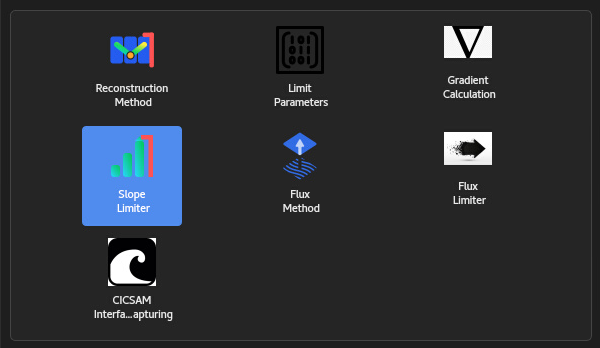
The slope limiter computes a local scalar multiplier
7.4.1 Limiter Activation
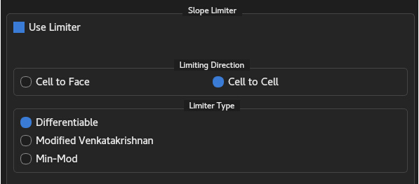
Use Limiter: Enabling slope limiting is strongly recommended for virtually all CFD simulation setups. Disabling the limiter (
unconditionally across the domain) leaves the higher-order spatial reconstruction completely unclipped. In the presence of local gradient spikes or mesh irregularities, unclipped reconstructions frequently induce non-physical numerical oscillations, directly leading to numerical divergence and solver failure.
7.4.2 Limiting Direction
The limiting direction determines the spatial neighborhood used to establish local maximum and minimum variable bounds during limiter evaluation:
Cell to Cell: Computes upper and lower variable bounds strictly from adjacent cell-center values across neighboring element centroids. Because cell-to-cell distances encompass a broader spatial stencil, this approach enforces tighter, more conservative clamping on local gradients. Consequently, Cell to Cell provides maximum numerical stability and robustness, making it the preferred choice for complex or poorly conditioned meshes.
Cell to Face: Evaluates bounds using extrapolated face-center values directly on the control volume boundaries. Because face-based bounds are spatially closer to the cell centroid and less restrictive, Cell to Face limiting applies less numerical damping to spatial gradients. While this preserves sharper peak gradients, it noticeably reduces overall solver robustness and increases susceptibility to local unsteadiness on skewed meshes.
7.4.3 Limiter Types
The mathematical formulation of the limiter dictates the smooth or sharp nature of gradient clipping. The available limiters are ordered below according to their limiting aggressiveness and dissipation levels, from the most restrictive to the least restrictive:
Differentiable Limiter:
Characteristics: Utilizes a smooth, continuously differentiable limiting function. Applies the highest level of gradient clamping among all available options.
Impact: Provides maximum numerical dissipation and optimal linear convergence behavior, making it highly robust for strongly coupled steady-state flows or severe non-linearities.
Modified Venkatakrishnan Limiter:
Characteristics: A widely established smooth limiter formulation that incorporates a threshold parameter to avoid active limiting in smooth flow regions while smoothly constraining extreme local peaks.
Impact: Delivers a balanced compromise between numerical dissipation and spatial accuracy, offering excellent convergence stalling prevention in general aerodynamics.
Min-Mod Limiter:
Characteristics: Implements a classic non-smooth TVD limiter function that selects the minimum absolute slope among neighboring cells if signs match, or zeroes out the gradient if signs differ. Represents the least dissipative (least limiting) scheme in the group.
Impact: Preserves sharp local gradients and peak wave amplitudes with minimal artificial clipping.
7.4.4 Application in Unsteady and Vortex-Shedding Flows
In scale-resolving transient simulations—such as vortex-shedding past bluff bodies, unsteady shear layer instabilities, Large Eddy Simulation (LES), Scale Adaptive Simulation (SAS) or Detached Eddy Simulation (DES)—excessive numerical dissipation can artificially damp transient physical eddies.
In these specific unsteady flow scenarios, utilizing the Min-Mod limiter in conjunction with Bounded Central Differencing (BCD) spatial reconstruction is particularly important. This combination minimizes numerical dispersion and artificial viscosity, allowing fine-scale transient turbulent vortices to shed and propagate naturally without triggering solution divergence.
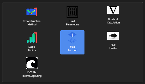
7.5 Flux Methods
Convective flux evaluation schemes compute the mass, momentum, and energy transport across control volume faces by solving approximate Riemann problems or utilizing flux-vector splitting formulations. Selecting an appropriate scheme is essential for accurately capturing acoustic waves, shock discontinuities, contact surfaces, and boundary layer shear profiles across various flow regimes.

7.5.1 AUSM+-up Scheme
Numerical Formulation: The Advection Upstream Splitting Method Plus Upstream (
-up) decouples convective transport (scalar advection) from acoustic wave propagation (pressure forces). It introduces Mach-number-dependent polynomial scaling functions along with pressure and velocity dissipation terms to eliminate numerical stiffness as the local Mach number approaches zero. Pros:
All-Speed Capabilities: Seamlessly operates across all flow regimes—from incompressible/low Mach number flows (
) up to high-speed supersonic and hypersonic flows ( ) without requiring preconditioning. Boundary Layer Resolution: Completely immune to the non-physical "carbuncle phenomenon" on blunt-body shock waves while maintaining low numerical dissipation inside viscous boundary layers.
Cons: Slightly higher computational complexity per face flux evaluation compared to basic flux-vector splitting schemes.
Recommended Usage: Default and highly versatile scheme for compressible aerodynamics, low-Mach thermodynamic flows, and high-speed shock-boundary layer interaction simulations.
7.5.2 HLLC Scheme
Numerical Formulation: The Harten-Lax-van Leer-Contact (HLLC) scheme is a three-wave approximate Riemann solver. Unlike the basic HLL solver, HLLC explicitly restores the intermediate contact discontinuity wave (
), dividing the Riemann fan into two acoustic wave bounds and a central contact surface. Pros:
Sharp Discontinuity Resolution: Delivers exceptional accuracy in resolving contact surfaces, density interfaces, temperature jumps, and material boundaries.
Robust Shock Capturing: Provides clean, non-oscillatory resolution of strong shock waves and rarefaction fans in transient compressible flows.
Cons: Can suffer from numerical carbuncle anomalies or grid-aligned shock instability in hypersonic bow shock regions unless additional entropy fixes are applied. Shows higher numerical dissipation in low-Mach boundary layers compared to
-up. Recommended Usage: Strongly recommended for high-speed compressible flows, transient shock tube phenomena, shock-expansion wave systems, and strong density-gradient fields.
Note. Phase Applicability Warning: The flux methods configured in this panel govern the convective flux calculations strictly for the continuous gaseous phase. If a dispersed multiphase model is active, the corresponding flux scheme for the particulate or droplet phase must be configured separately under
PhysicsDispersed PhaseFlux Method.
Note. Interface Availability Notice: Although the Flux Limiter Tool and CICSAM Interface Capturing Tool options are visible within the GUIX-H user interface, they are currently inactive and inaccessible in the present software release.