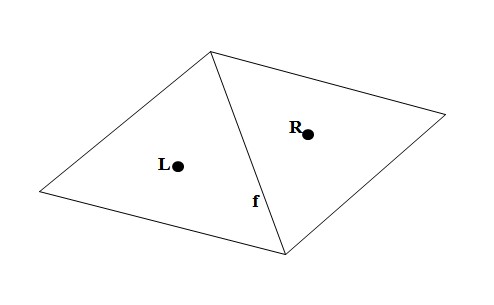
6 Carrier Flux Discretization on Interior Faces

6.1 Face geometry and orientation

Consider an interior face \(f\) shared by cells \(L\) and \(R\). The unit normal \(\mathbf{n}_f\) is oriented from \(L\) to \(R\) and the area is \(A_f\). A conservative numerical flux must satisfy the orientation identity \[\mathbf{F}(\mathbf{q}_L,\mathbf{q}_R,\mathbf{n}_f) =-\mathbf{F}(\mathbf{q}_R,\mathbf{q}_L,-\mathbf{n}_f), \](6.1) so that the same face contribution enters neighbouring cells with opposite sign.

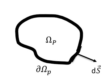
Finite-volume control volume sketch — Figure 6.1: Finite-volume control volume and outward differential surface element used in the integral conservation statements.

Interior face geometry with left and right cells — Figure 6.2: Interior-face geometry with left and right cell locations used for flux reconstruction.

6.2 Compressible AUSM-family flux

For a compressible aerodynamic state, an AUSM-family inviscid face flux can be separated into a numerical mass flux and mechanical pressure, \[\mathbf{F}_f^c= \begin{bmatrix} \dot m_f\\ \dot m_f\mathbf{u}_{\mathrm{up}}+p_f\mathbf{n}_f\\ \dot m_f H_{\mathrm{up}} \end{bmatrix}, \](6.2) with appended turbulence/species components transported by the appropriate numerical mass flux. AUSM⁺-up constructs \(\dot m_f\) from split Mach functions and a pressure-difference correction, and constructs \(p_f\) from split pressure functions and a velocity-difference correction (Liou 2006). This separation is valuable for a primitive-variable coupled solver because pressure-to-continuity and velocity-to-momentum couplings appear directly in the face Jacobian.

For a moving/rotating coordinate representation the convective normal speed is formed relative to the grid/frame velocity. The energy flux must then be derived consistently for the selected absolute- or relative-energy formulation. The current implementation status of this term is discussed in Chapter 20.

6.3 Constant-density artificial-compressibility flux

For the incompressible regime, the pressure-index row is the numerical mass flux rather than a density flux. The current row structure is \[\mathbf{F}_f^{ac}= \begin{bmatrix} m_fu_{1,\mathrm{up}}+p_fn_1\\ \vdots\\ m_fu_{d,\mathrm{up}}+p_fn_d\\ m_f\\ m_fH_{\mathrm{up}} \end{bmatrix}, \](6.3) where \(m_f\) is mass flux per unit area. Turbulence and species rows use the same \(m_f\). Because the physical density is constant, pressure influences continuity through the AUSM⁺-up pressure-difference correction and through the pseudo-time pressure coefficient, not through an equation-of-state derivative \(\partial\rho/\partial p\).

6.4 Viscous momentum flux

The viscous momentum flux is \[\mathbf{F}_{m,f}^{v}=\boldsymbol{\tau}_f\cdot\mathbf{n}_f,\] with \(\boldsymbol{\tau}\) from Eq. (2.4). On an unstructured cell-centred grid, \(\nabla\mathbf{u}\) is reconstructed at the face. For non-orthogonal grids a simple two-point normal difference is insufficient by itself; the reconstruction must retain the tangential/non-orthogonal gradient contribution used by the active CMPS gradient path.

6.5 Energy and species diffusion

The viscous/thermal energy flux contains heat conduction and, where enabled, viscous work and species enthalpy diffusion, \[F_{E,f}^{v} = (\boldsymbol{\tau}_f\cdot\mathbf{u}_f)\cdot\mathbf{n}_f -\mathbf{q}_f\cdot\mathbf{n}_f -\sum_s h_s\mathbf{J}_{s,f}\cdot\mathbf{n}_f.\] The exact active terms depend on solver options and material/species configuration. A dependent-species formulation requires the enthalpy-diffusion correction to be constructed consistently with Eq. (2.6).

6.6 AD face Jacobian

For each face, the complete expression is differentiated with respect to both cell states, \[\delta(\mathbf{F}_fA_f) =\mathbf{J}_{f,L}\delta\mathbf{q}_L +\mathbf{J}_{f,R}\delta\mathbf{q}_R.\] For cell \(L\), these derivatives are accumulated into its diagonal and \(R\)-neighbour matrix blocks. For cell \(R\), the same conservative face flux is assembled with opposite orientation. This produces the block-sparse nearest-neighbour coupling used by the global implicit solver.

6.7 HLLC carrier flux

The current compressible carrier solver also contains an HLLC flux path. CMPS forms density-weighted Einfeldt-type left and right signal estimates. With face-normal velocities \(u_{n,L}\) and \(u_{n,R}\), the Roe-like normal velocity and acoustic estimate are

\[\bar u_n=\frac{\sqrt{\rho_L}u_{n,L}+\sqrt{\rho_R}u_{n,R}}{\sqrt{\rho_L}+\sqrt{\rho_R}},\]

\[a_f^2=\frac{\sqrt{\rho_L}a_L^2+\sqrt{\rho_R}a_R^2}{\sqrt{\rho_L}+\sqrt{\rho_R}} +\frac12\frac{\sqrt{\rho_L\rho_R}}{(\sqrt{\rho_L}+\sqrt{\rho_R})^2}(u_{n,R}-u_{n,L})^2.\]

The bounding wave speeds are \(S_L=\bar u_n-a_f\) and \(S_R=\bar u_n+a_f\). The contact speed is determined from pressure and momentum continuity across the star region, and the final HLLC flux selects the left, left-star, right-star or right state according to the signs of \(S_L\), \(S_*\) and \(S_R\). Species are convected with the selected mass flux. The homogeneous VOF production path currently uses the AUSM carrier flux rather than HLLC.

Writing the implementation wave estimates explicitly, with \(q_L=\sqrt{\rho_L}\) and \(q_R=\sqrt{\rho_R}\),

\[S_L=\bar u_n-a_f,\qquad S_R=\bar u_n+a_f.\]

The contact-wave speed used by the current carrier HLLC path is

\[S_*=\frac{(p_R-p_L)+\rho_Lu_{n,L}(S_L-u_{n,L})-\rho_Ru_{n,R}(S_R-u_{n,R})}{\rho_L(S_L-u_{n,L})-\rho_R(S_R-u_{n,R})}.\]

The common star pressure obtained from the left state is

\[p_*=p_L+\rho_L(S_L-u_{n,L})(S_*-u_{n,L}),\]

and the star density on side \(K\in\{L,R\}\) is

\[\rho_{*,K}=\rho_K\frac{S_K-u_{n,K}}{S_K-S_*}.\]

In vector form, the HLLC flux is selected piecewise as

\[\mathbf F_{HLLC}=\begin{cases}\mathbf F_L,&0\le S_L,\\ \mathbf F_{*,L},&S_L\le0\le S_*,\\ \mathbf F_{*,R},&S_*\le0\le S_R,\\ \mathbf F_R,&S_R\le0.\end{cases}\]

For transported species, the star-region species flux follows the HLLC mass flux and the upwind mass fraction, so conservation of total carrier mass and constituent mass remains tied to the same contact wave.