2 Graphical User Interface (GUI)
2.1 GUIX-H and NeuralFlow Hierarchy and Inter-Process Communication
As established in the architectural hierarchy outlined in Section 1.3.1, the operational framework of the software relies on a strict supervisor-worker paradigm where the GUIX-H process maintains absolute control over the underlying computational layers. To maintain complete user-interface responsiveness and prevent computational heavy-lifting from lagging the frontend, the communication between the graphical interface and the active solvers is handled entirely via an optimized, low-latency Inter-Process Communication (IPC) network layer.
Within this framework, a single, centralized GUIX-H process is fully capable of managing, orchestrating, and monitoring multiple independent NeuralFlow solver processes running concurrently on local or distributed high-performance computing hardware nodes. Each individual NeuralFlow instance spawned by the supervisor communicates with the master interface through a dedicated network interface utilizing a precise allocation of exactly four distinct TCP/IP ports.
By decoupling these network streams across four independent ports per solver instance, GUIX-H can cleanly isolate vital control commands from high-bandwidth visualization data, ensuring that the user interface retains instant responsiveness and rigid process control even during intense, massive scale multiphase CFD calculations.
Within this supervisor-worker paradigm, the graphical interface maintains absolute operational authority over all spawned computational instances, offering three distinct tiers of runtime process control:
Process Spawning and Initialization: Through the configuration panel, GUIX-H can instantiate a brand-new, independent NeuralFlow solver process by passing runtime parameters such as mesh dimensionality and parallel execution arguments. Upon triggering, the interface invokes the exact native binary, provisions the necessary operating system resources, and automatically binds the four-port IPC network architecture to establish a secure initial handshake.
Connect and Disconnect: The interface allows users to dynamically attach to any running NeuralFlow solver to extract real-time convergence data and visual field monitoring. Conversely, users can safely disconnect the GUI frontend from the solver process; this leaves the backend computational loop running uninterrupted in the background while freeing up local interface memory.
Graceful Termination: Through the control panel, GUIX-H can transmit a structured interrupt signal to a specific solver process. This prompts NeuralFlow to cleanly finalize its current iteration, execute an automated save of the current solution vectors to prevent data loss, and execute a controlled shutdown.
Operating System Kill: In scenarios involving severe numerical stagnation, unrecoverable matrix freezes, or user-initiated aborts, GUIX-H can bypass standard application protocols and issue low-level Operating System (OS) force-kill commands. This immediately terminates the targeted NeuralFlow process and instantly reclaims allocated CPU cores and system RAM.

Operational Note: All spawned solver instances are cataloged in a centralized table visible within the Solvers tab of the GUIX-H interface, located at the very top of the tab. In order to execute any of the process management operations described above (connect, disconnect, graceful termination, or OS kill) on a specific solver instance, the user must first explicitly select the target solver row from the table to focus the command context.
Simulation Naming Constraint: To maintain workspace data integrity and prevent directory path conflicts, two distinct NeuralFlow solver processes sharing the exact same "Simulation Name" identifier cannot coexist or execute simultaneously. Each spawned instance must be assigned a unique naming attribute to ensure proper log segregation, file tracking, and communication routing within the GUIX-H supervisor layer.
2.2 User Interface Components
2.2.1 File Menu
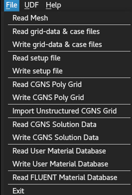
The File Menu serves as the primary data ingestion, storage, and configuration gateway for the GUIX-H interface, managing all external file interactions for computational grids, solver cases, and thermodynamic databases.
2.2.1.1 Read Mesh
Imports discretized volumetric configurations. Supported external
file extensions include native formats and Fluent-compatible mesh grids
(.msh) generated by ANSYS Meshing or ANSYS Fluent. In
alignment with the solver’s predefined parsing constraints, this
operation is strictly limited to ASCII-encoded formats;
binary-formatted meshes cannot be ingested.
2.2.1.2 Read/Write Grid-Data & Case Files
Performs a comprehensive batch I/O operation that simultaneously
loads or writes the entire simulation state. This includes the CGNS
poly-grid topology, the corresponding numerical solution data file
(.cgns) housing the independent primitive variables, and
the associated case setup file (.neuralflow).
2.2.1.3 Read/Write Setup File
Loads or exports the simulation control profile (.neuralflow)
independently of the mesh. This file retains all user-defined physical
models, cell zone attributes, solver controls, and boundary condition
states, allowing users to restore the exact environment configuration
without reloading heavy grid files.
2.2.1.4 Read/Write CGNS Poly Grid
Handles the isolated reading or writing of the poly computational
grid layout. The poly grid definition is stored and managed
co-dependently with the active simulation state vectors within the
standardized .cgns file format.
2.2.1.5 Import Unstructured CGNS Grid
[Technical Description Pending] Reserved for importing alternative unstructured CGNS grid topologies. This feature establishes the structural translation layer for non-polyhedral grid formats (detailed specifications will be provided in a future release update).
2.2.1.6 Read/Write CGNS Solution Data
Handles the standalone loading or writing of the converged numerical
state vectors (independent primitive variables). This dataset is
securely archived alongside the underlying geometric configuration
within the standardized .cgns architecture.
2.2.1.7 Read/Write User Material Database
Opens or saves custom thermophysical and transport property libraries
using the native NeuralFlow material database format (.mdb),
enabling the reuse of standardized fluid or solid definitions across
different simulation projects.
2.2.1.8 Read FLUENT Material Database
Parses and imports legacy or external fluid/solid material property
libraries directly from the ANSYS Fluent Scheme-based database format
(.scm).
2.2.1.9 Exit
Safely terminates the active GUIX-H graphical user interface process.
2.2.2 UDF Menu
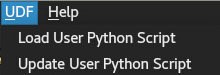
The UDF (User-Defined Function) Menu provides the interface framework required to inject custom user-written scripts into the simulation environment, enabling the definition of dynamic runtime parameters and non-standard physical behaviors.
2.2.2.1 Load User Python Script
Enables users to browse and load an external Python script
(.py) containing user-defined execution logic. In transient
formulations, this script is ingested by the framework to evaluate
time-dependent boundary conditions and dynamically manipulate the
time-step size at the start of each temporal iteration through custom
Python methods.
2.2.2.2 Update User Python Script
Synchronizes and hot-reloads the modified runtime logic of an already loaded Python script directly into the active NeuralFlow solver memory. This allows users to apply real-time script corrections, algorithmic adjustments, or boundary-state refinements to the underlying backend computational loop without requiring a full re-initialization of the simulation workspace.
2.2.3 Help Menu
The Help Menu provides users and developers with direct access to comprehensive technical documentation, theoretical background resources, and software metadata essential for verifying solver behavior and exploring code structures.

2.2.3.1 Theory Guide
Provides direct access to the comprehensive theoretical reference manual in PDF format. This document details the mathematical foundations of the NeuralFlow solver, including the governing fluid-dynamics and multi-phase equations, spatial and temporal discretization schemes, boundary condition formulations, and numerical convergence algorithms.
2.2.3.2 Code Documentation
Launches an interactive, browser-based HTML documentation suite compiled directly from the in-code developer comments. This reference resource maps the underlying object-oriented architecture of the software, detailing the C++ class hierarchies, inheritance trees, member functions, and individual class member variables to facilitate backend development and codebase exploration.
2.2.3.3 About
Triggers a graphical pop-up window within the interface that displays general diagnostic and metadata information for the NeuralFlow suite. This dialog presents the current software release version, active build configurations, copyright details, and a high-level overview of the application’s core capabilities.
2.2.4 Workflow Toolbar
The Workflow Toolbar serves as the central operational backbone of the GUIX-H interface. It is architected as a sequential, step-by-step pipeline that guides the user chronologically through the entire preprocessing, solver configuration, execution, and post-processing phases of a Computational Fluid Dynamics (CFD) simulation. By organizing the simulation setup into logical, left-to-right functional tabs, the toolbar minimizes configuration errors and ensures a streamlined engineering workflow.

2.2.4.1 Solvers Toolbar
Acts as the process management control center. It allows users to spawn new NeuralFlow solver instances, monitor active simulation runs, and dynamically control the connection, disconnection, or termination states of various backend computational processes linked to the master GUIX-H interface.
2.2.4.2 Grid Toolbar
Manages the import, manipulation, and diagnostic verification of the
computational mesh. Key capabilities include reading fresh mesh files,
performing bidirectional conversions between 2D planar and 2D
axisymmetric configurations, and exporting grid quality metrics. For 2D
axisymmetric simulations, it provides automated spatial translation
tools to shift the coordinate system of the computational grid directly
to the radial axis of symmetry (
2.2.4.3 Physics Toolbar
Governs the activation of physical models and temporal formulations. Users can select between steady-state and transient time-marching schemes and activate the specific physical modules required for the simulation, such as turbulence closure models, dispersed-phase multiphase formulations, and chemical species transport. It also exposes control parameters and physical coefficients associated with these active modules.
2.2.4.4 Materials Toolbar
Serves as the thermodynamic and physical property registry for the simulation. It catalogs all active fluid, solid, particle, and mixture materials. Users can import standardized material profiles from predefined databases directly into the active solver context or manually customize transport and state properties (such as density, viscosity, and thermal conductivity) to fit specialized simulation needs.
2.2.4.5 Zones Toolbar
Manages the volumetric subdomain definitions imported with the mesh. This panel catalogs all volumetric cell zones, allowing users to designate their physical state (such as fluid or solid subdomains) and pair them with the appropriate material definitions registered in the active case file.
2.2.4.6 B.C. Toolbar
Controls the enforcement of mathematical boundary states on the computational domain boundaries. It registers all face zones defined within the mesh file, enabling the user to assign specific boundary condition types (such as inlets, outlets, or walls) and define their respective hydrodynamic, thermal, or chemical boundary values.
2.2.4.7 Numerics Toolbar
Exposes the underlying spatial and temporal discretization controls of the solver. Users can configure the high-order spatial reconstruction methods, define physical upper and lower clipping limits for independent primitive variables to maintain solver stability, choose gradient calculation techniques, select slope limiters, and specify the approximate Riemann flux solver to resolve cell-face interface fluxes.
2.2.4.8 I.C. Toolbar
Manages the initialization of the flow field. The panel catalogs all volumetric cell zones, allowing the user to specify distinct, zone-specific initial conditions (such as localized pressure, temperature, or phase fraction patches) to establish a physically realistic starting state before commencing the primary calculation.
2.2.4.9 Monitor Toolbar
Defines the runtime data logging, diagnostic tracking, and automated backup schedules. This panel allows users to configure the auto-save frequency, define surface and boundary zones for automated export into the VTU file format, configure spatial point probes or surface reports for transient tracking, and customize convergence parameters for residual plots and console printouts.
2.2.4.10 Solution Control Toolbar
Houses the execution and numerical stability parameters of the
solver. Users can configure the CFL number, maximum iteration limits,
physical time-step sizes (
2.2.4.11 Solve Pushbutton
A high-priority interactive pushbutton that acts as the immediate simulation trigger. It allows users to instantly launch the numerical calculation, pause the iteration loop to evaluate intermediate results, or gracefully halt/stop the active run without losing computed state vectors.
2.2.4.12 Postprocess Toolbar
Provides localized spatial visualization and data extraction tools directly within the interface. It displays a list of face sections and surface boundaries alongside their associated flow-field variables. Users can render custom-scaled color contours of converged variables, generate 2D cutting planes (slices) through 3D geometries, extract linear data profiles between two user-defined coordinate points (line plots), and compute surface integrals over designated boundaries to extract integral parameters like mass flow rates or heat fluxes.