4 Physical Properties
Built-in Material Database Support:
To streamline the simulation setup, NeuralFlow includes a native,
pre-populated material database by default. This internal registry
contains standardized, validated thermophysical property profiles for
6 fluid materials, 4 solid materials,
and 4 particle materials, which can be instantly loaded
into the case file without manual parameter entry.
Aerospace Modeling Recommendation:
For high-speed external aerodynamic applications involving Conjugate
Heat Transfer (CHT), the extreme kinetic energy dissipation within the
boundary layer yields significantly elevated adiabatic wall
temperatures. Under these severe thermodynamic conditions, it is highly
recommended to select the Gupta curves formulation or
Sutherland’s law depending on the wall temperature to
evaluate the temperature-dependent thermal conductivity (
4.1 Defining a New Material
The NeuralFlow framework grants users the operational flexibility to define completely customized material profiles from scratch. Users can manually specify thermodynamic, transport, and structural properties for three distinct material categories: fluids, solids, and discrete particles.
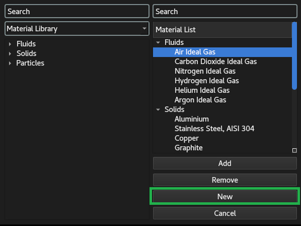
Depending on the chosen category, the interface exposes specific property fields and numerical formulation models:
Fluid Materials:
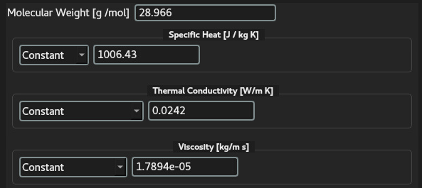
Fluid Material Properties Specific Heat (
): Constant, Polynomial, or Piece-wise Polynomial. Thermal Conductivity (
): Constant, Polynomial, Piece-wise Polynomial, or Kinetic Theory formulations. Viscosity (
): Constant, Polynomial, or Piece-wise Polynomial.
Solid Materials:
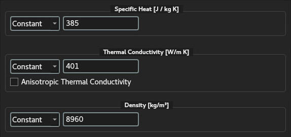
Solid Material Properties Specific Heat (
): Constant, Polynomial, or Piece-wise Polynomial. Thermal Conductivity (
): Constant, Polynomial, or Piece-wise Polynomial. Density (
): Constant, Polynomial, or Piece-wise Polynomial.
Particle Materials:
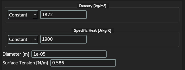
Particle Material Properties Density (
): Constant, Polynomial, or Piece-wise Polynomial. Specific Heat (
): Constant, Polynomial, or Piece-wise Polynomial. Diameter (
): Strictly limited to Constant values. Surface Tension (
): Strictly limited to Constant values.
It should also be underlined that temperature unit used defining a polynomial material property is K.
Once all material properties have been accurately and completely specified, the user can click the Create button to officially register the custom material within the NeuralFlow framework; and you can see the defined material with the given name at the material list.
CRITICAL WORKFLOW RECOMMENDATION: Custom Material Generation
Please note that the feature enabling the creation of completely new materials from empty templates has undergone limited validation and testing in the current release. The primary, verified user workflow relies on utilizing the built-in default library or importing predefined material datasets directly into the active case context. To ensure absolute numerical stability and prevent parsing discrepancies, users are strongly discouraged from constructing entirely new materials from scratch. It is highly recommended to satisfy simulation requirements by reading and modifying an existing, verified material database instead.
4.2 Changing Existing Material Properties
Users can define any material property using either constant values or temperature-dependent polynomial formulations. These settings can be configured during the initial case setup or modified as needed before/during execution. Even if an imported material database lacks pre-defined polynomial coefficients for a specific substance, users can still manually introduce polynomial definitions for any desired thermal property directly within GUIX-H.
To modify or switch property formulations, select the target substance from the Material List inside the Materials Tool. The property model (e.g., switching between constant and polynomial) can be selected using the adjacent combo box, while individual numerical values and coefficients can be edited directly via the corresponding line edit fields.
Important Note: Applying Material Property Changes
Upon completing any modifications to a material’s properties, the user must click the Apply Changes button to transmit the updated parameters to the NeuralFlow solver. If this step is omitted, the changes will remain restricted strictly to the GUIX-H interface, and the solver will continue running with the previously registered material parameters.
Anisotropic Thermal Conductivity for Solid
Materials:
For advanced structural thermal configurations, NeuralFlow supports the
definition of directional heat conduction through an anisotropic thermal
conductivity formulation. This allows setting direction-dependent
thermal responses modeled as a structural second-order tensor:
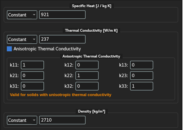
When populating this tensor, users must strictly adhere to the following numerical and spatial constraints:
Scaling Coefficient Multiplier Behavior: The numerical entries populated within the anisotropic thermal conductivity tensor act strictly as dimensionless scaling coefficients (multipliers). The effective thermal conductivity along a given principal axis is determined by multiplying the baseline isotropic thermal conductivity value (which can be configured as a constant, polynomial, or piece-wise polynomial function) by the corresponding directional tensor coefficient (
, , or ) specified in the matrix. Thermal Conductivity Tensor Usage: The underlying energy solver exclusively evaluates the principal diagonal components of the tensor, specifically
( -direction), ( -direction), and ( -direction). Off-diagonal cross-coupling coefficients are strictly neglected and have no impact on the thermal conduction routines. Dimensionality Constraints for 2D Cases: In 2D planar or axisymmetric simulation formulations, the spanwise thermal conductivity component
( -direction) is entirely redundant and is completely bypassed during the spatial discretization and flux evaluation phases.
4.3 Material Database File Formats
To facilitate the rapid, consistent, and automated loading of thermophysical properties across different simulation cases, the NeuralFlow solver and GUIX-H interface support the use of structured, external material database files. Instead of manually inputting property polynomials, kinetic theory constants, and state-dependent parameters for every new simulation run, users can archive complete material catalogs in portable files.
At present, the framework natively supports two distinct material database file formats. Both formats allow for the complete representation of fluid, solid, and discrete-phase (particle) materials, including custom temperature-dependent curve fits. However, they differ in their syntactic structure, human-readability, and ease of automated manipulation through external scripting.
These two supported file formats are detailed comprehensively in the following subsections:
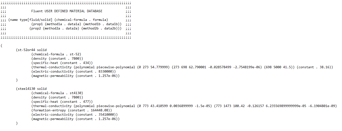
4.3.1 ANSYS Fluent Material Database
An example of ANSYS Fluent Scheme-based database format
(.scm) is given below.
4.3.2 User Material Database
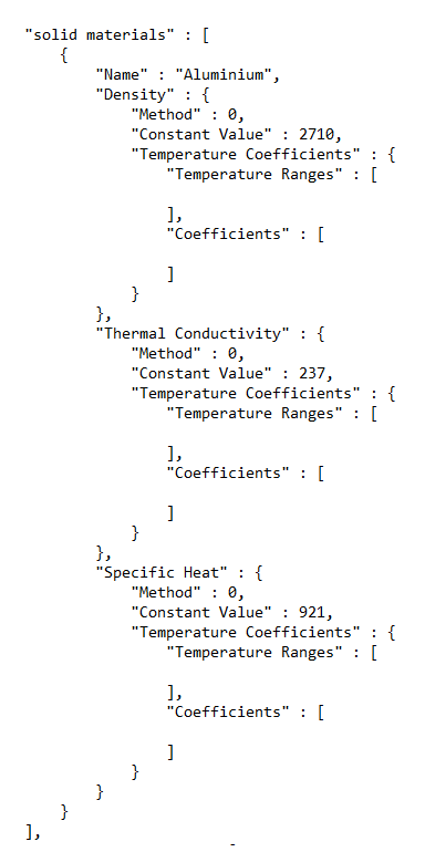
NeuralFlow natively supports its own custom material database format
structured in JSON (JavaScript Object Notation). An example
of NeuralFlow JSON-structured database format (.mdb) is given
below.
4.4 Reading Material Database
To load an existing material database into the simulation workspace, users can utilize the dedicated import utilities located within the main menu bar of the application. The graphical user interface provides separate file-reading routines specifically tailored to parse and validate the two supported database formats:
ANSYS Fluent Material Database: To ingest a standard Fluent-formatted database, navigate to:
File
Read FLUENT Material Database This executes a specialized parser optimized to read the standard LISP-like Scheme syntax utilized by ANSYS Fluent material database files.
User Material Database: To load a custom or user-defined material catalog, navigate to:
File
Read User Material Database This option triggers the generic reader designed to parse user-defined database structures.
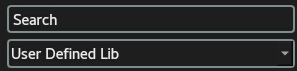
Upon selecting either menu path, a standard system file browser dialog will appear, prompting the user to locate and select the target database file. Once the file is successfully parsed without errors, the imported substances can be accessed within the Material Tool by selecting User Defined Lib from the library selection combo box. This action displays a structured list containing all the materials parsed from the database, neatly categorized by their respective material types (Fluids, Solids, and Particles), enabling the user to easily load them into the active case context as described in Section 4.5.
Use Case Note: Locating Substances in Large Databases
When working with exceptionally large material databases, locating a specific substance from the extensive catalog can become challenging. To address this, the interface features an integrated search utility situated directly above the library selection combo box. By typing the name (or a partial string) of the target substance into this Search field, the matching entries are instantly highlighted within the Material Library list, enabling rapid identification and selection.
4.5 Loading and Managing Case Materials
To utilize any substance from the built-in library within a simulation, the material must first be loaded into the active case context. This step transitions the material from the global database into the active session’s local memory, making it available for physical assignments.
The workflow for managing active case materials involves the following operations:
Loading Materials to the Case: The user can browse the global Material Library, select the desired substance, and click the Add button. This action duplicates the material profile and appends it to the active Material List. Only the substances present in this active list can be utilized in the boundary conditions or domain settings of the current simulation.
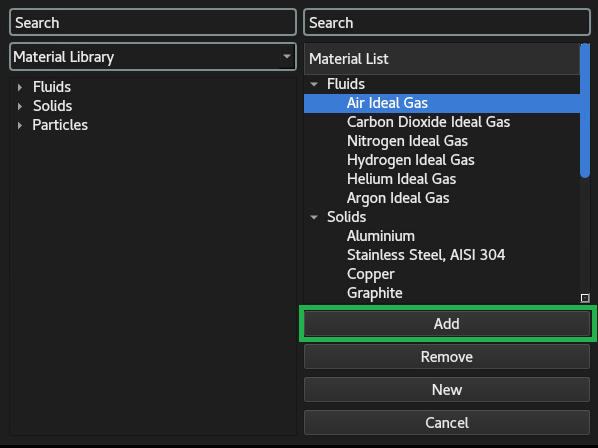
Adding a Material from Material Database Modifying Case Materials: Once a material has been successfully loaded into the Material List, its thermophysical, transport, or structural properties can be dynamically edited at any point to meet specific simulation requirements without altering the master database.
Removing Materials: If a loaded substance is no longer needed in the simulation setup, it can be selected from the active list and discarded by clicking the Remove button. Note that the solver will block the removal of any material that is currently bound to an active cell zone or boundary condition.
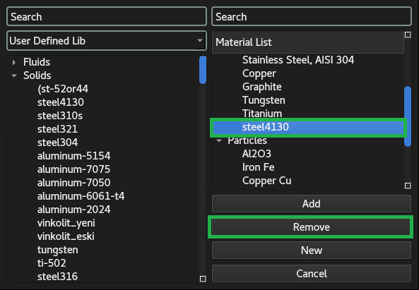
Removing a Material from Case
Important Workflow Clarification: Transferring a material from the global library to the active Material List merely registers it within the active case file; it does not automatically assign the substance to any volumetric region of the grid. To bind a loaded material to a physical domain, the user must explicitly configure the cell zone settings as detailed in Section 5.2.