13 Autosave Data
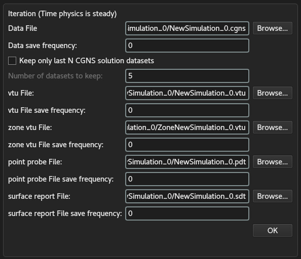
The Autosave Options Tool, accessible via the Monitor Tool menu, provides automated periodic exporting of computational solution data, post-processing visualization fields, localized probes, and surface-integrated diagnostics during solver execution. The interface shown in Figure 13.1 allows users to specify file destinations and output frequencies independently for each data category.
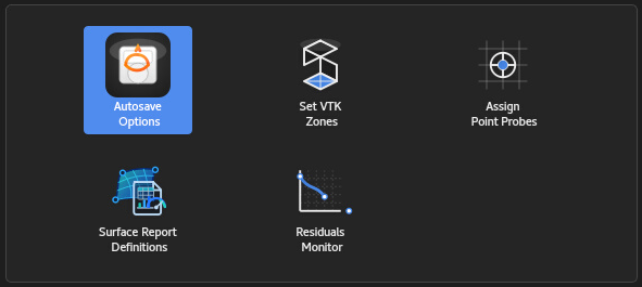
13.1 Saving Solution Data File
Primary simulation state data is exported in standard CGNS
(.cgns) format. The solution data file stores the complete
set of primitive variables across the entire computational domain,
serving as the primary checkpoint for solver restart and
continuation.
13.1.1 File Structure and Dataset Management
To optimize input/output (I/O) efficiency, the CGNS polygrid mesh topology is written to the file once during initialization. Subsequent solution states are appended directly to this base file structure as time steps or iteration counts progress.
13.1.2 Dataset Truncation Option
Users can manage disk storage by enabling the Keep only last
N CGNS solution datasets option and specifying the retention
depth (
Steady-State Analyses: Retaining only the last
datasets (e.g., ) is highly recommended to cap disk footprint while preserving recent convergence history. Transient Analyses: Truncation is not recommended for unsteady simulations, as discarding intermediate time steps prevents reconstructing time-accurate unsteady flow evolution.
13.2 Saving Domain VTU File
NeuralFlow outputs binary unstructured VTK XML files (.vtu)
mapping scalar and vector fields across the global domain. These files
enable comprehensive 3D post-processing and visual analysis in
open-source platforms such as ParaView or commercial tools like Ansys
EnSight.
Memory and Storage Caution: Domain VTU files contain the full volumetric mesh and all active solution variables. Consequently, file sizes can be substantial. Setting an excessively small vtu File save frequency (e.g., saving every iteration) can rapidly exhaust available disk storage and induce I/O bottlenecks.
13.3 Saving Zone VTU File
To avoid the large storage overhead of global domain files, users can
configure Zone VTU Files (.vtu) restricted
exclusively to designated boundary or internal zones.
13.3.1 Setting VTU Zones
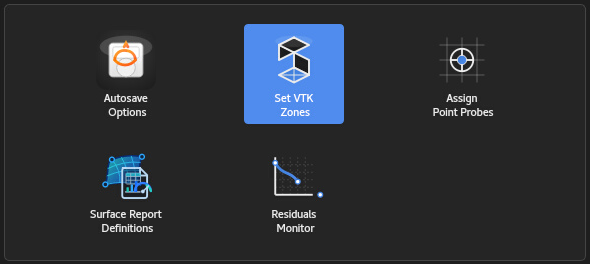
To designate specific boundary boundaries or surface regions for targeted post-processing export, users configure the zone selection table within the interface (Figure 13.4).
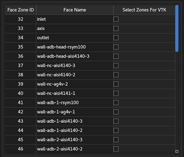
The interface lists all physical boundary boundaries defined within
the domain topology, displaying their unique Face Zone
ID alongside their descriptive Face Name
(e.g., inlet, outlet, axis, and
various solid wall boundaries).
Users explicitly select which boundaries to export by checking the corresponding entries under the Select Zones For VTU column.
13.3.2 Dimensionality Reduction
Zone-based exporting extracts reduced-dimensional sub-geometries:
3D Simulations: Exports 2D surface meshes for selected wall, inlet, or outlet boundaries.
2D Simulations: Exports 1D boundary line segments.
This targeted output drastically reduces file size while streamlining post-processing for localized phenomena, such as surface pressure distributions, boundary layer shear stress, or shock-wall interactions.
13.4 Saving Point Probe File
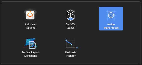
Point probes allow localized time-series tracking of dependent and
independent flow variables at specified spatial coordinates within the
computational domain. Probes export formatted ASCII text files
.pdt.
13.4.1 Real-Time Monitoring and Diagnostic Plotting
Point probe data can be monitored dynamically during execution:
Console Output: Real-time probe variable values can be printed directly to the Message View screen.
Live Plotting: Variable histories (e.g., pressure fluctuations, temperature decay) can be rendered as real-time line plots against iteration count or physical time.
13.5 Saving Report Definition File
Surface Report Files .sdt log
surface-integrated quantities, flux balances, physical properties, and
aerodynamic forces across specified boundary zones (defined via Surface
Definitions).
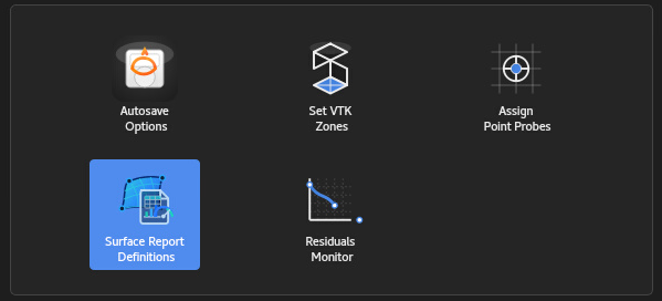
The surface reporting features allow evaluation across three distinct report types:
Surface Integral: Computes dependent or independent solution variables over selected surfaces using the following averaging methods:
Area-Weighted Average
Mass-Weighted Average
Force Report: Evaluates forces, moments, and aerodynamic coefficients based on a specified Reference Pressure [Pa]:
Pressure Force
Shear Force
Total Force
Center of Pressure
Drag Coefficient (
) Lift Coefficient (
) Moment
Note: Calculating the Center of Pressure and Moment requires defining the Reference Axis.
Flux Report: Quantifies transport properties passing through a designated boundary:
Mass Flux
Particle Mass Flux
Mass Flow Rate
Particle Mass Flow Rate
Heat Flux
13.5.1 Adding a Surface Definition
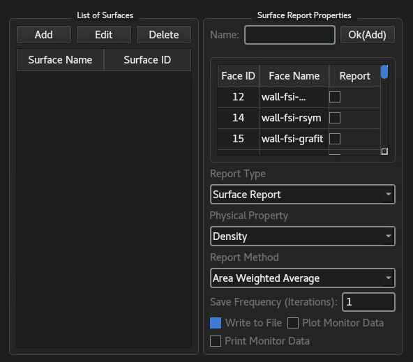
To create a new surface diagnostic metric, click the Add button located above the List of Surfaces panel. This action activates the input fields within the Surface Report Properties panel.
The step-by-step procedure for adding a surface report is as follows:
Assign Name: Enter a unique descriptive identifier in the Name field.
Select Target Surfaces: Highlight the desired boundary surfaces from the face list by checking the corresponding boxes under the Report column.
Choose Report Type: Select the primary diagnostic category from the Report Type drop-down menu (Surface Report, Force Report, or Flux Report).
Specify Physical Property: Select the target flow variable to be evaluated (e.g., Density, Static Pressure, Velocity) via the Physical Property menu.
Set Report Method: Where applicable, specify the integration or averaging scheme (e.g., Area Weighted Average, Mass Weighted Average) from the Report Method drop-down menu.
Configure Output Options: Set the desired Save Frequency (Iterations) and toggle output options such as Write to File, Plot Monitor Data, and Print Monitor Data.
Confirm Definition: Click the Ok(Add) button to finalize setup.
Upon confirmation, the newly defined surface metric is automatically registered in the List of Surfaces table, populated with its assigned Surface Name and generated Surface ID.
13.5.2 Editing a Surface Definition
To modify the parameters of an existing surface report:
Select the target surface entry from the List of Surfaces table.
Click the Edit button located above the surface list. The current configurations of the selected item will populate the Surface Report Properties panel.
Make the necessary modifications (e.g., changing physical properties, adjusting evaluation methods, or toggling plot options).
Click the Ok(Edit) button to update and commit the changes.
13.5.3 Deleting a Surface Definition
To permanently remove a surface diagnostic entry from the monitoring workflow:
Highlight the surface definition to be removed within the List of Surfaces table.
Click the Delete button above the surface list.
Confirm the deletion action by clicking the Ok(Delete) button in the Surface Report Properties panel.
Once confirmed, the selected definition is erased from the List of Surfaces table, and all associated file writing, dynamic plotting, and console logging routines for that metric are deactivated.
13.5.4 Surface Diagnostics and Convergence Verification
Users can define arbitrary surface metrics—including mass flow rate,
area-weighted pressure, heat flux, or force components (
Streaming integrated quantities to the Message View console for immediate verification.
Dynamic plotting of integrated quantities versus iteration or time steps to monitor global flow convergence and periodic steady-state behavior.
13.6 Residual Monitoring and Data Plotting
Real-time tracking of equation residuals is essential for assessing numerical stability and determining global solution convergence. The Residual Monitoring panel (Figure 13.9) controls the visual rendering, console logging, scaling behavior, and inter-process communication frequency between the core solver engine (NeuralFlow) and the graphical user interface (GUIX-H).
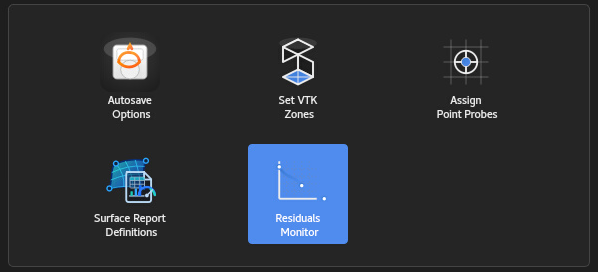
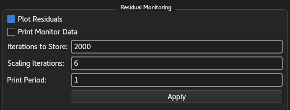
The interface provides the following configuration options:
Plot Residuals: Enables dynamic, real-time graphical rendering of conservation equation residuals (e.g., continuity, momentum, energy, species) within the active plotting window.
Print Monitor Data: Toggles formatted numerical residual output, streaming step-by-step convergence data to the console message view and solver log file.
Iterations to Store: Specifies the maximum iteration history buffer retained and rendered in the residual plot window. For long-running steady-state simulations, this caps memory consumption by discarding older data points while maintaining a clear view of recent convergence trends.
Scaling Iterations: Defines the initial iteration window used to calculate the residual normalization factors. Raw unscaled residuals computed during these baseline iterations are averaged to scale subsequent residual values, providing a relative measure of order-of-magnitude reduction.
Print Period: Sets the iteration interval for transferring residual data and monitoring metrics from NeuralFlow to GUIX-H. All active line plots and printed console metrics refresh strictly according to this specified step frequency.
Performance Note / Communication Overhead:
In simulations featuring very small grid sizes or executed across high core-count parallel environments, per-iteration compute times can be extremely short. Under these conditions, transferring residual data to the interface at every iteration (Print Period = 1) may introduce noticeable inter-process communication (IPC) overhead between NeuralFlow and GUIX-H. To eliminate performance bottlenecks and maximize overall solver throughput, it is highly recommended to increase the Print Period (e.g., to 5 or 10 iterations).