NeuralFlow Theory & User Reference Manual › User's Guide › Modeling Basic Fluid Flow

NeuralFlow User's Guide v2.0 — Chapter 6

6 Modeling Basic Fluid Flow

This chapter describes the basic physical models that NeuralFlow provides for fluid flow. In NeuralFlow, all fluid flows are fundamentally modeled and solved as compressible flows. At present, there is no support for incompressible flow formulations. As a direct consequence, the baseline fluid flow model in NeuralFlow—when no viscous or advanced physical models are activated—corresponds to a compressible inviscid flow solution (governed by the compressible Euler equations).

When a mesh file is successfully imported and all setup parameters are left in their default states, the solver defaults to a steady, laminar simulation utilizing air modeled as an ideal gas with constant transport and thermophysical properties (for a 2D domain, a planar solution space is set as default).

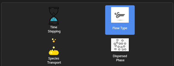
By navigating to the Physics Tool and explicitly configuring the Flow Type setting to Inviscid, the user establishes the most fundamental fluid flow model executable within NeuralFlow.

6.1 Physics of Compressible Flows

Compressible aerodynamic flows are fundamentally characterized by stagnation (total) quantities, specifically total pressure and total temperature . For an ideal gas, the relationship between these total properties and their static counterparts ( and ) is generally defined via the temperature-dependent specific heat :

When assuming a constant specific heat ratio (), Equation 6.1 simplifies into the classical isentropic relations governed by the local Mach number and the specific heat ratio :

6.1.1 Flow Regimes and Choking Dynamics

Equations 6.2 and 6.3 dictate how local thermodynamic properties vary as fluid velocity changes under ideal, reversible (isentropic) conditions. In one-dimensional flow analysis, these equations allow the direct determination of the local Mach number provided the total-to-static pressure ratio is known.

Key physical phenomena described by these formulations include:

Choked Flow Condition: For air (), the critical static-to-total pressure ratio at which sonic velocity () is achieved equals . This choked condition typically occurs at the location of minimum cross-sectional area (e.g., a nozzle throat). For typical solid propellant combustion products (), this calculation yields a critical pressure ratio of .
Diverging Section Behavior: Downstream of the throat, the flow trajectory depends on the exit pressure:
- It can continue accelerating to supersonic speeds, characterized by a continuous decline in static pressure.
- It can return to subsonic flow, decelerating while experiencing a pressure recovery (rise in static pressure).
Shock Wave Formation: If a supersonic stream is subjected to an imposed adverse pressure gradient (backpressure), an abrupt non-isentropic transition occurs through a shock wave, resulting in a sudden jump in static pressure accompanied by rapid deceleration.

6.2 The Compressible Form of the Ideal Gas Law

For compressible flow simulations in NeuralFlow, the fluid density () is dynamically coupled to the thermodynamic state of the gas through the compressible formulation of the ideal gas law:

where the parameters are defined as follows:

is the global reference operating pressure.
is the local static pressure relative to the operating pressure (i.e., gauge pressure, making the absolute static pressure ).
is the universal gas constant.
is the molecular weight of the active fluid medium.
is the local static temperature, which is evaluated directly from the solution of the energy equation.

Note on Operating Pressure:
In NeuralFlow, the operating pressure is fixed at zero (). Consequently, all static pressure values defined in boundary conditions or computed by the solver directly represent absolute pressures, making the gauge pressure and absolute pressure values identical ().

6.3 Time Formulation and Preconditioning Options

NeuralFlow supports both Steady and Transient time-marching formulations. Because density-based coupled solvers inherently suffer from severe numerical stiffness in low-Speed or mixed-speed flow regimes (), advanced preconditioning techniques are integrated to optimize convergence performance across both steady and time-accurate simulations.

6.3.1 Time Marching Formulations

Steady Formulation: Solves for the asymptotic steady-state solution by integrating the governing conservation equations in pseudo-time (): where represents the spatial residual vector and is the preconditioning matrix. Local Time Stepping (LTS) is used to accelerate convergence by computing a distinct pseudo-time step () for each cell based on the user-specified CFL number, local cell geometry, and local acoustic/convective wave speeds: where is the cell volume and represents the spectral radius of the convective flux Jacobians.
Transient Formulation: Resolves physical time-accurate phenomena (). To maintain high physical accuracy while avoiding small time-step limitations, NeuralFlow utilizes a Dual Time-Stepping approach. At each physical time step , an inner pseudo-time iteration loop () is solved to drive the physical residual to zero: This formulation guarantees second-order temporal accuracy (BDF2) while enabling the use of preconditioning during inner pseudo-time iterations.

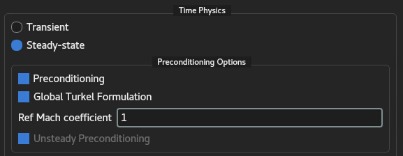
Time Marching Formulations and Preconditioning Options

6.3.2 Preconditioning Options

In standard density-based formulations, as the local Mach number approaches zero (), the speed of acoustic waves () becomes orders of magnitude larger than the convective fluid velocity (). This disparity causes the condition number of the system matrix to approach infinity (), resulting in slow residual decay and poor pressure-velocity coupling. Preconditioning rescales the pseudo-acoustic wave speeds to match the local convective velocity magnitude, restoring the matrix condition number to .

6.3.2.1 Preconditioning

When enabled (ON), the solver premultiplies the pseudo-time derivative by the preconditioning matrix . This option is critical for low-Mach subsonic flows, low-speed regions within compressible domains (e.g., boundary layers, recirculation zones, stagnation chambers), and conjugate heat transfer interfaces. Disabling (OFF) reverts the solver to standard density-based time marching, which is recommended only for purely supersonic/hypersonic flows () where acoustic and convective wave speeds are naturally comparable.

6.3.2.2 Global Turkel Formulation (ON / OFF)

Implements the modified Turkel preconditioning matrix formulation. The Turkel transformation alters the pressure derivatives in the energy and momentum equations via a dynamic scaling parameter : The Global variant ensures global stability across complex unstructured meshes by evaluating reference scales smoothly, preventing localized mathematical singularities near stagnation points () and sonic transitions (). Maintaining this option ON ensures optimal numerical stability and seamless integration across subsonic, transonic, and supersonic zones.

6.3.2.3 Reference Mach Coefficient

Controls the scaling sensitivity of the preconditioned reference velocity : where is the Reference Mach Coefficient.

Value = 1.0 (Default): Provides the ideal theoretical balance between acoustic wave speed equalization and matrix conditioning.
Values : Increases artificial acoustic wave speed, adding numerical dissipation to damp strong transient oscillations at the expense of slightly slower low-Mach convergence.
Values : Increases preconditioning aggressiveness in extremely low-speed recirculation zones.

6.3.2.4 Unsteady Preconditioning

In time-accurate transient simulations, applying standard preconditioning directly to physical time derivatives destroys physical time accuracy. The Unsteady Preconditioning algorithm applies the preconditioning matrix strictly to the inner pseudo-time iterations () within the dual time-stepping framework while leaving physical time derivatives () unconditioned.

6.3.2.4.1 Key Benefits:

Retains full physical time accuracy () for transient vortex shedding, acoustics, and unsteady combustion.
Accelerates inner loop pseudo-time convergence per physical time step by 3x to 5x, significantly reducing total computation time per physical second.
Automatically active (ON) by default when switching to the Transient time formulation.

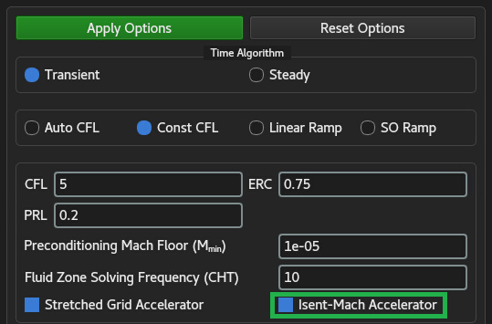
6.4 Isentropic Mach Accelerator (`Isent-Mach Accelerator`)

The Isentropic Mach Accelerator is an advanced preconditioning enhancement algorithm designed to accelerate global solver convergence in internal flow domains characterized by vast spatial variations in pressure and velocity. A classic example includes solid propellant rocket motors (SRMs) and converging-diverging nozzles, where the combustion chamber exhibits high total pressure () at very low speeds (), transitioning rapidly to sonic () at the throat and supersonic () in the expansion section.

6.4.1 Physical Motivation and Continuity Stiffness

In density-based coupled solvers, pseudo-time marching equations are preconditioned to equalize the convective and acoustic wave propagation speeds. Standard local preconditioning (e.g., Weiss-Smith or Turkel formulations) computes the artificial acoustic speed based strictly on local velocity magnitudes: where is the local speed of sound, is the local velocity magnitude, and is the preconditioning floor.

In domains with severe pressure ratios (), such as solid rocket motor chambers, in the stagnation region is extremely small. Using standard local preconditioning causes a severe disparity between the pseudo-acoustic time scale of the high-pressure chamber and the high-velocity nozzle. Consequently, pressure updates stall, mass conservation (continuity) residuals iterate slowly, and global convergence deteriorates significantly.

6.4.2 Mathematical Formulation

The Isentropic Mach Accelerator resolves this continuity stiffness by dynamically scaling the local preconditioning parameter using the local isentropic Mach number , derived directly from the local total-to-static pressure ratio: where is the local (or domain-referenced) total pressure, is the static pressure, and is the specific heat ratio.

By incorporating into the preconditioning matrix , the modified pseudo-acoustic reference velocity becomes: where is an adaptive weighting coefficient.

6.4.3 Mechanism of Acceleration

Pseudo-Acoustic Wave Speed Alignment: By estimating the expansion potential of the fluid via , pseudo-time pressure disturbances in high-pressure, low-speed zones travel significantly faster. This eliminates the bottleneck in mass flux equilibration.
Continuity Residual Flushing: Similar to coupled continuity convergence accelerators, it couples static pressure corrections directly with the downstream throat expansion capability, rapidly driving global continuity residuals down without requiring smaller global time steps (CFL).
Seamless Transition: In regions where local flow velocity matches the expansion state (such as the nozzle throat and supersonic plume), , smoothly reverting the preconditioning matrix back to standard density-based formulations with zero numerical penalty.

6.4.3.0.1 Usage Recommendation:

The Isent-Mach Accelerator option is strongly recommended for internal compressible flow simulations featuring high-pressure stagnation chambers, rocket motor grain channels, safety relief valves, and complex expanding nozzles. Enabling this feature typically yields a 10x to 30x speedup in total solver iterations required to achieve residual convergence.