5 Cell Zone and Boundary Conditions
5.1 Supported Cell Zone Types
The NeuralFlow solver features advanced numerical capabilities designed to model complex Conjugate Heat Transfer (CHT) problems, where thermal energy is dynamically exchanged across fluid-structure interfaces. To facilitate this coupled thermodynamic behavior, the framework is engineered to solve not only conventional fluid dynamics but also solid-state thermal conduction.
Consequently, computational domains imported into GUIX-H must be partitioned into one of two supported cell zone classifications:
Fluid
Solid
5.2 Changing Cell Zone Types
The Zones configuration panel, accessible directly via the Workflow Toolbar, provides a centralized tabular interface designed to manage the physical classification and material properties of all volumetric subdomains (cell zones) imported with the computational grid.
This panel displays a structured database listing of all active cell zones alongside their key topological and physical attributes:
ID: The unique numerical index assigned to the specific cell zone during the grid generation or mesh parsing phase.
Name: The alphanumeric string identifier associated with the zone.
Type: The current modeling classification of the volumetric zone, which designates it as either a Fluid or a Solid domain.
Material: The active thermodynamic material or multi-phase mixture currently bound to the zone.
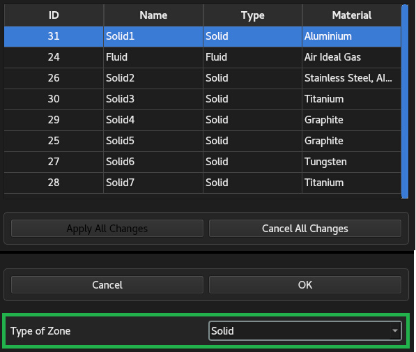
Within this interactive table, the user can select any specific cell zone row to dynamically configure its properties. Through the integrated editing controls, the operator can alter the zone classification (converting a zone from Fluid to Solid, or vice versa) using a dedicated type-selection combo box. Additionally, a zone name can be edited by double-clicking on its name on Cell Zone List.
5.3 Assigning Material to a Cell Zone
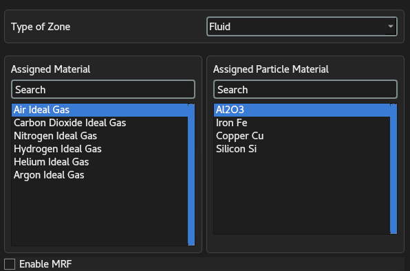
The physical substances assigned to these zones are managed through a dynamic integration with the Materials panel, where materials are either custom-defined or imported from the pre-created material database into the active case context. These registered case materials then populate the material selection list within the Zones panel. To prevent configuration errors, this list is fully context-sensitive: the interface automatically filters and displays the available materials based on the selected zone type (Fluid or Solid) while simultaneously accounting for the active physical models enabled in the simulation (such as species transport or dispersed-phase formulations). The operator can then assign the desired material from this dynamically filtered list, ensuring instant synchronization with the backend solver.
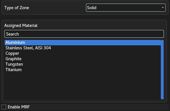
As shown in Figure 5.3, the user must assign a particle material to the fluid zone when dispersed-phase model is activated.
5.3.0.0.1 Note:
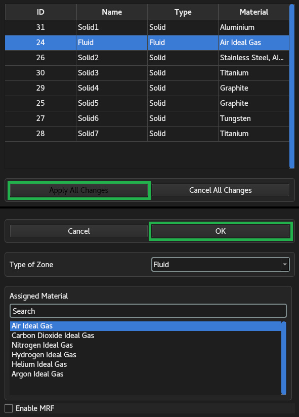
Following any modification within a cell zone, both the OK and Apply All Changes buttons must be clicked sequentially:
OK Button: Commits the applied changes locally within the GUIX-H user interface.
Apply All Changes Button: Transmits the updated zone types and assigned materials across all cell zones from GUIX-H to the NeuralFlow solver.
5.4 Supported Boundary Condition Types
Boundary conditions define the essential mathematical and physical constraints at the external and internal interfaces of the computational domain. In NeuralFlow, these conditions are managed and modified via the B.C. Tool located on the Workflow Toolbar.

The B.C. Tool automatically parses and displays all boundary zones defined within the imported mesh file, organized in a structured table containing the following properties:
BC Zone ID: The unique numerical identifier associated with the specific boundary zone in the native mesh file.
BC Name: The alphanumeric name assigned to the boundary during the grid generation process.
BC Type: The physical boundary condition classification imported from the mesh file.
Modifying Boundary Names and Types:
Users can easily customize the boundary configuration using the
following interactive workflows:
Renaming a Boundary: Double-click directly on the target row within the BC Name column to enter inline editing mode, type the new name, and press Enter to save.
Changing a Boundary Type: Select the target boundary row from the table and use the Boundary Condition Type combo box to assign a new physical classification.
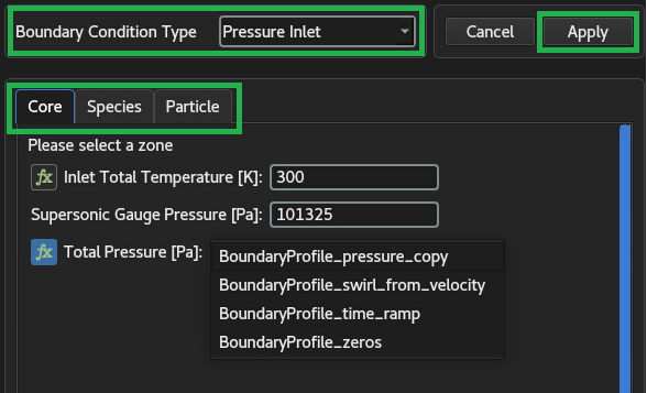
Upon changing the boundary type, the interface dynamically updates to expose the required parameter input fields. These are organized into dedicated tabbed panels:
Core Tab: Automatically becomes visible upon type selection to capture the primary physical parameters (e.g., velocities, pressures, temperatures).
Species and Particle Tabs: If advanced physics models—such as species transport or dispersed-phase (particle) models—are active in the case, the corresponding Species Tab and Particle Tab are enabled alongside the Core Tab. Users must carefully review and populate these supplemental tabs to prevent incomplete setup errors.
Important Note: Applying Boundary Condition Changes
Upon completing any modifications to a boundary, the user must click the Apply button to transmit the updated conditions to the NeuralFlow solver. If this step is omitted, the changes will remain restricted strictly to the GUIX-H interface, and the solver will continue running with the previously registered boundary conditions.
5.4.1 Overview of Supported Boundary Types
The NeuralFlow framework supports a comprehensive suite of boundary types designed for complex fluid, solid, and multi-phase applications:
Wall: Applied to physical solid boundaries bounding the fluid domain.
Velocity: Supports the definition of a constant wall velocity for moving boundaries.
Thermal Boundary Conditions: Users can configure the wall’s thermal behavior using one of the following models:
Adiabatic Wall: Zero heat flux normal to the wall.
Constant Temperature: A fixed, uniform temperature boundary.
Convective Heat Transfer: Models external convection using a heat transfer coefficient and wall ambient temperature.
Constant Heat Flux: A fixed, uniform thermal energy input per unit area.
External Radiation: Models radiative heat transfer to/from an external environment using wall ambient radiation temperature and wall emissivity.
External Mixed: A combined formulation accounting for both convection and external radiation simultaneously.
Coupled Wall (FSI): Used for fluid-structure interaction (FSI) and conjugate heat transfer (CHT) boundaries where physical states are dynamically coupled across adjacent cell zones. It can only be enabled when a the boundary is two-sided, i.e. the boundary has to be located at the two different cell zones. The heat transfer through that boundary can also be enabled/disabled; so it can also act as an adiabatic wall.
Mass Flow Inlet: Specifies a fixed mass flow rate and total temperature at the inflow boundary.
Pressure Outlet: Defines a static pressure condition and backflow total temperature at the outflow boundary. Within this configuration, the solver allows the user to choose between two numerical pressure enforcement methods:
Forced: A rigid Dirichlet-type boundary formulation where the user-specified static pressure (and backflow temperature, if reverse flow occurs) is strictly and uniformly imposed directly on the boundary faces.
Interpolated: The default formulation where boundary face pressures are dynamically reconstructed by interpolating values from the adjacent interior cell centers to the boundary faces. This allows local pressure gradients to develop naturally across the outlet plane rather than forcing a completely uniform pressure distribution. This numerical treatment significantly improves convergence stability, naturally accommodates non-uniform velocity profiles exiting the domain, and prevents non-physical acoustic wave reflections at the exit boundary, especially where the boundary is in supersonic regime.
Farfield: Applied to external flow boundaries to model free-stream conditions, with free-stream Mach and static temperature conditions with the flow direction.
Pressure Inlet: Specifies total pressure and temperature at the flow inlet.
Solid Propellant: Dedicated to reactive boundaries using the classical empirical burning rate relation:
where is the linear burning rate, is the burn rate coefficient, is the local pressure, and is the pressure exponent. Axis: Used as the centerline boundary for axisymmetric computational domains.
Symmetry: Applies a zero-gradient, mirror-image boundary condition across symmetry planes.
Important Workflow Clarification: Interior Zones
Because interior cell zones (Fluid Interior and Solid Interior) are defined within the mesh file structure, they will also appear in the boundary condition list. However, due to the integrated workflow of GUIX-H, any modification made to the cell zone types within the Zones Tool (as described in Section 5.2) is automatically propagated to this list. Therefore, users do not need to manually change or configure interior zone types within the B.C. Tool.
5.4.1.0.1 Tip: Boundary Condition Duplication
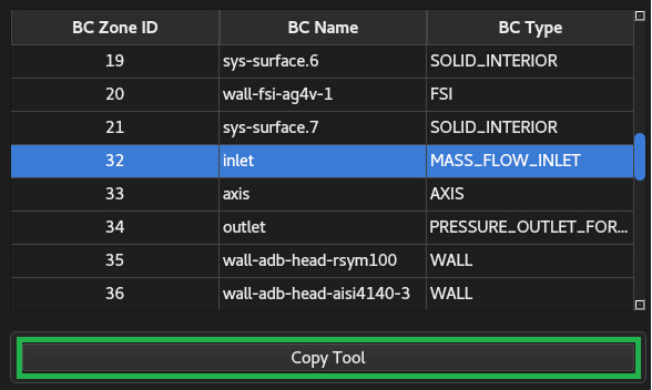
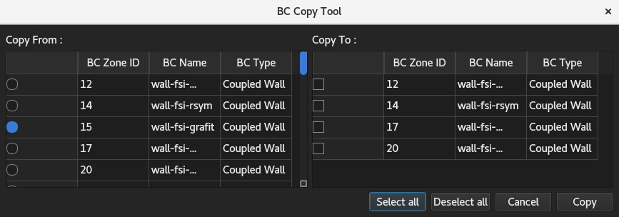
Configuring each boundary individually in complex solution domains with numerous boundaries can lead to setup errors and excessive pre-processing time. Using the Copy Tool integrated into the B.C. Tool, boundary conditions assigned to a reference boundary can be quickly applied to target boundaries sharing the same boundary type, ensuring consistency and expediting case preparation.
5.5 Using User-Defined Functions (UDF) for Boundary Conditions
In transient flow applications, specifying static boundary values is
often insufficient to capture the dynamic, time-varying physics of the
system. To address this limitation, NeuralFlow features an embedded Python
interpreter, allowing users to define and deploy time-dependent
User-Defined Functions (UDFs) instead of relying strictly on constant
boundary inputs. Any field value required by a boundary condition—such
as static pressure, Mach number, or temperature—can be parameterized as
a function of physical time (
The implementation, linking, and management of custom Python scripts follow a structured workflow within the application:
5.5.1 Script Initialization and Structure
Whenever a new computational process or project is initialized within NeuralFlow, the framework automatically creates a directory named pyScripts inside the designated project Working Directory. Inside this folder, a template Python file named UserScripts.py is generated by default.
Users can open this script using any text editor to construct arbitrary Python functions. These functions should compute and return the desired boundary parameter value based on the simulation’s progress. The details of how to write a user-defined Python function is detailed in Chapter 16.
5.5.2 Loading and Linking UDFs in the GUI
To register and apply these custom functions within the active simulation setup, the operator must execute the following procedure:
Load the Script: Navigate to the main menu and select:
UDF Menu
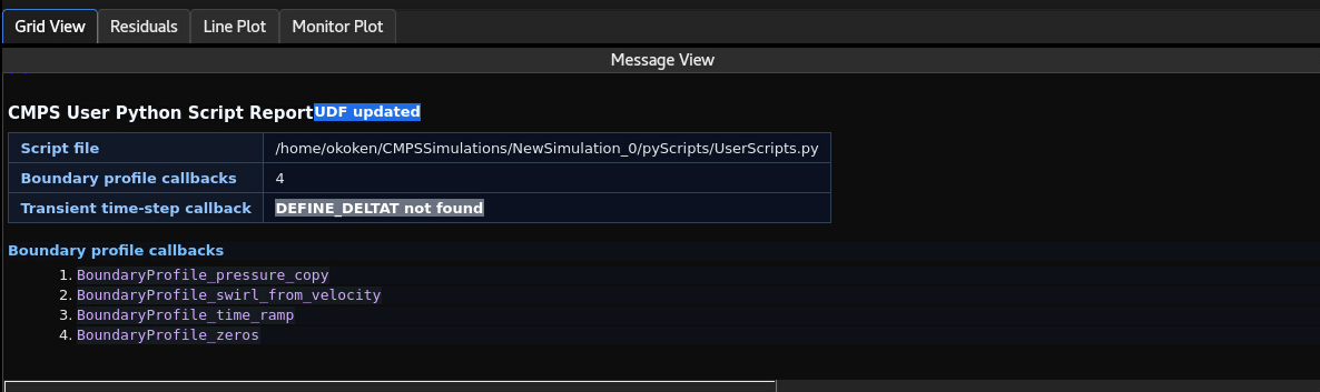
Load User Python Script This registers the target Python file with the embedded interpreter. When a UDF script is successfully loaded, key details and parsed function summaries are automatically reported to the Message Window:
Script File: Displays the full absolute path of the loaded Python script file.
Boundary Profile Callbacks: Reports the total number of available boundary profile functions identified within the script (i.e., the count of methods defined using the
DEFINE_PROFILEmacro).Transient Time-Step Callback: Reports the total number of custom time-step size functions defined within the script (i.e., the count of methods defined using the
DEFINE_DELTATmacro).Boundary Profile Callbacks List: Provides an itemized list of the exact function names of all parsed and available boundary profiles.
Activating UDF for a Boundary Condition Link to Boundary Conditions: Within the parameter input panels of the B.C. Tool, each input field features an adjacent fx (function) button. Clicking this button enables UDF mode for that specific boundary value and allows the user to link the parameter to a designated Python function parsed from the loaded script.
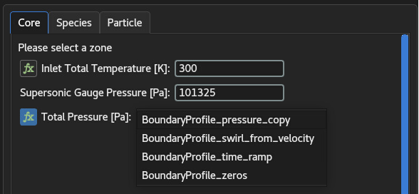
Activating UDF for a Boundary Condition
Once linked, the backend solver queries the specified Python function at every physical time step, automatically updating the boundary condition value as the simulation progresses.
5.5.3 Hot-Reloading and Dynamic Updates
If a user modifies the Python script (e.g., altering a coefficient or equation) while the simulation setup is active, the embedded interpreter must be notified to register these changes. Rather than reloading the entire project, the user can navigate to:
UDF Menu
This action instantly hot-reloads the Python runtime environment, parsing the updated script and applying the modified logic to the active boundary conditions immediately.
Workflow Safety and Validation Note: To prevent runtime solver failures, NeuralFlow automatically executes a static validation and syntax check whenever the Load User Python Script or Update User Python Script routines are triggered. If any syntax errors or invalid Python structures are detected, the GUI intercepts the loading process, flags the issue, and alerts the user with a detailed diagnostic warning. While this automated check prevents corrupt scripts from entering the system, users must still ensure that their custom functions do not introduce logical runtime errors and strictly return numerical values corresponding to the physical units expected by the target boundary field.
For a comprehensive guide, detailed programmatic syntax examples, and advanced implementation strategies regarding custom UDF design, please refer to Chapter 16.